Cong Li, Jianshe Lei (2014). Numerical tests for effects of various parameters in niching genetic algorithm applied to regional waveform inversion. Earthq Sci 27(5): 541-551. DOI: 10.1007/s11589-014-0095-7
Citation:
Cong Li, Jianshe Lei (2014). Numerical tests for effects of various parameters in niching genetic algorithm applied to regional waveform inversion. Earthq Sci 27(5): 541-551. DOI: 10.1007/s11589-014-0095-7
Cong Li, Jianshe Lei (2014). Numerical tests for effects of various parameters in niching genetic algorithm applied to regional waveform inversion. Earthq Sci 27(5): 541-551. DOI: 10.1007/s11589-014-0095-7
Citation:
Cong Li, Jianshe Lei (2014). Numerical tests for effects of various parameters in niching genetic algorithm applied to regional waveform inversion. Earthq Sci 27(5): 541-551. DOI: 10.1007/s11589-014-0095-7
In this paper, we focus on the influences of various parameters in the niching genetic algorithm inversion procedure on the results, such as various objective functions, the number of the models in each subpopulation, and the critical separation radius. The frequency-waveform integration (F-K) method is applied to synthesize three-component waveform data with noise in various epicentral distances and azimuths. Our results show that if we use a zero-th-lag cross-correlation function, then we will obtain the model with a faster convergence and a higher precision than other objective functions. The number of models in each subpopulation has a great influence on the rate of convergence and computation time, suggesting that it should be obtained through tests in practical problems. The critical separation radius should be determined carefully because it directly affects the multi-extreme values in the inversion. We also compare the inverted results from full-band waveform data and surface-wave frequency-band (0.02-0.1 Hz) data, and find that the latter is relatively poorer but still has a higher precision, suggesting that surface-wave frequency-band data can also be used to invert for the crustal structure.
The 1-D velocity crustal model in a region is one of the most concerned scientific issues for our seismologists, because a suitable 1-D model can produce reasonable earthquake location, seismic moment tensor inversion, and 3-D velocity structure by seismic tomography (Begnaud et al. 2000). Usually, a 1-D crustal velocity model is obtained by summarizing the results inferred from deep seismic soundings and receiver function analysis (e.g., Li et al. 2008; Zhang and Wang 2009; Mishra and Zhao 2003; Lei et al. 2009, 2014; Lei 2011, 2012). However, deep seismic soundings and receiver function analysis can only provide the crustal structure along a specific seismic line or under certain stations, which suggests that our obtained 1-D model cannot fully reflect the crustal structure in the entire study region. The regional waveform inversion technique is regarded as an effective tool, because its results contain more information of deep structure in both travel time and waveform along good-coverage paths from events to seismic stations under the region, and it has been frequently used in recent years (e.g., Dreger and Helmberger 1990; Rodgers and Schwartz 1998; Du and Panza 1999; Li et al. 2007, 2012).
Waveform inversion is a general non-linear optimization solver but with highly non-uniqueness (Maurice et al. 2003; Wang 2014). However, traditional inversion techniques, such as conjugate gradient method, grid search method, genetic algorithms, and simulated annealing method, usually can only generate one minima (Bina 1998; Stoffa and Sen 1991). Niching genetic algorithms (NGA) can efficiently produce the multi-minimal for multi-parameters by simulating the evolutionary process in biology. With the help of some operators like crossover, mutation, selection, and competition, NGA inversion can converge to different minima effectively and thus is widely used in seismology. Koper et al. (1999) further developed the NGA and inverted for source parameters of the earthquakes occurred in Kuril Islands. Using the waveform data and technique of NGA, Maurice et al. (2003) inferred the crustal and upper mantle structure of southernmost South America. Li et al. (2012) applied the NGA to the waveform data and inferred the 1-D crustal structure under southeastern Gansu, China. However, few researchers investigate the accuracy of velocity structure from NGA waveform inversion and effects of different objective functions, number of models in each subpopulation, and critical separation radius on the deduced velocity structure, but these parameters are vital to the NGA waveform inversion. In this paper, we illustrate how these parameters affect the resulting velocity model.
2.
Methodology
In some previous studies, NGA is based on crowding (e.g., De Jong 1975) or sharing scheme (e.g., Goldberg 1989; Goldberg and Richardson 1987). In the first case, every parent models will be compared randomly with several children models in a given subpopulation. The children models which are the most similar to the parent model will be weeded out. After certain generations, all models that share similar "gene" will be deleted, promoting the diversity in "gene" as most as possible and allowing different subpopulations to inhabit different searching niches (Mahfoud 1995). Different from crowding scheme, NGA with sharing scheme is accomplished by distributing a sharing function to every models in a certain subpopulation. This sharing function is defined by similarities between different models and will reduce the fitness value of each model. Thus, by evaluating the fitness values related to sharing function, the similar models will be eliminated in the NGA procedure. On the other hand, distinct models will converge to separate demes representing local minima (Holland 1975).
The NGA used in our present study is based on sharing function in nature, but differing from those described above, our NGA explicitly defines the number of subpopulation and models before the inversion. In this way, individual model will be artificially migrated to a given niche or area in model space, which represents the minima of objective function. This explicit definition avoids the possibility that subpopulation appears or disappears accidently owing to the stochastic searching (Koper et al. 1999). Although we cannot know how many minima could exist in the objective function before, we can determine it by several tests with critical separation radius, which we will discuss in later section.
The basic principle of our NGA is described as follows: Initially, all the models are divided into n subpopulations and each includes m models. In the first generation, the first subpopulation runs independently as the traditional genetic algorithm. Then, the second subpopulation runs as similar as first one except that every model in the subpopulation will be compared with the most optimal model in the first subpopulation. If the similarity between these two models is smaller than the given criterion, which is called a critical separation radius (Rc, defined in Sect. 4.3), the similar model in the second subpopulation will be weeded out in later running. Again, the procedure of the third subpopulation is the same as that of the second subpopulation except for being compared with the most optimal models in both the first and second subpopulations. Similarly, other subpopulations run until the n-th subpopulation's running is completed. The process is repeated until the generation reaches the value we preset.
The definition of the similarity between two models is the key to NGA. In our study, we define the similarity as follows:
where m represents the number of parameters we need search, xi and yi are the i-th parameters of models X and Y, Ai and Bi are the upper and lower bounds of the i-th parameters.
3.
Model parameterization
We first compute synthetic seismograms with different distances and azimuths in a given model. With these synthetic waveforms, we carry out numerical tests using different objective functions, number of models in each subpopulation, and critical separation radius so that we can focus on the effects of these parameters on the inversion results. Then, we check the reliability of the NGA waveform inversion result by comparing it with our given model.
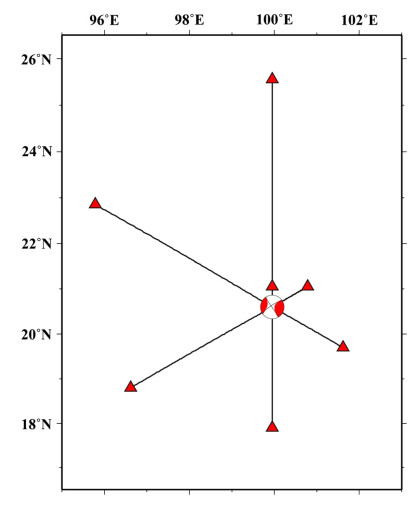
We choose a MW 5.0 earthquake that occurred in March 25, 2011 in Myanmar. The source depth and focal mechanisms (Table 1) are from Global CMT Catalog Search (http://globalcmt.org). The model is divided into 4 layers, sediment, upper crust, middle crust, and lower crust with the thickness of 5, 10, 15, and 15 km, respectively, and these layers correspond to P-wave velocities of 5.5, 6.0, 6.5, and 7.0 km s-1. The Pn-wave velocity is 8.0 km s-1. The vP/vS ratio is fixed as 1.732 so that the S-wave velocity can be determined. The density in each layer is computed according to the formula, ρ = 0.77 + 0.32vP (e.g., Berteussen 1977). The seven three-component synthetic waveforms are computed using the F-K (frequency-waveform integration) code (Zhu and Rivera 2002) with the distances of 50, 100, 200, 300, 400, 500, and 550 km and the azimuths of 0°, 60°, 120°, 180°, 240°, 300°, and 360° (Fig. 1).
Table
1.
Source parameters used in NGA waveform inversion
A total of 5 P-wave velocities and 4 thicknesses of layers will be searched. The searching ranges are within a range of ±0.5 km s-1 for P-wave velocity and ±25 % for the thickness around the preset values as described in Sect. 3. The NGA inversion is run for five times with 50 generations and 5 subpopulations. We average five results to be our final model and define deviation of 5 models as the error. Referring to previous results (Bhattacharyya et al. 1999), the probabilities of crossover and mutation are set as 0.85 and 0.12, respectively. Here, we mainly investigate how to determine some parameters in the NGA inversion, such as objective function, number of models in each subpopulation, and critical separation radius. In order to simulate the seismic wave close to real one as most as possible, synthetic seismograms containing different level of noise, signal-to-noise ratio (SNR), 10, 5, and 3 dB, are used in our NGA inversion. Note that because of the scope of the paper, here we only illustrate the results inferred from the synthetics with the SNR of 10 dB in the Sects. 4.1, 4.2, and 4.3, but we still discuss the effects of different SNRs on the results in the Sect. 4.4.
4.1
Objective function
Objective function is usually not definite in NGA inversion, but it is defined personally. However, different objective functions could have a great influence on the convergence and result of the inversion to some extent (Wang and Zhang 2006), hence which type of objective function is chosen is vital to the inversion result. According to previous studies (Bhattacharyya et al. 1999; Li et al. 2007), we designed three-types of functions in our present NGA. The first one is the average deviation of difference between the amplitudes of synthesized and observed seismogram, and it can be defined as follows:
(1)
where Oij and Sijare the amplitudes of observed and synthesized seismograms of the i-th component at the j-th sampling time, Nw represents the number of waveforms used in the inversion. The second one is the cross-correlation function between observed data and synthetic waveform, and its form can be described as follows:
(2)
where ci is the normalized cross-correlation coefficient between the i-th observed data and synthetic seismogram. Referring to Mellman (1980), the third objective function is related to the cross-correlation function but only get its value of the zero-th point, and its form is as follows:
(3)
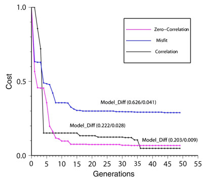
The time evolution of cost value for these three objective functions in the most optimal subpopulation is presented in Fig. 2. The precision of inversion results of different objective functions are evaluated by following formulas:
Figure
2.
Cost versus generations. Results from NGA inversions with different objective functions, deviation of difference in the amplitudes (blue), cross-correlation function (black), and zero-th-lag cross-correlation function (pink). The two numbers in the bracket after Model_Diff represent the average errors for thickness (in km) and velocity (in km/s), respectively
where Hi and Vi are the inverted thickness and P-wave velocity in the i-th layer, hi and vi are corresponding given values. Comparing with the results of other two functions (Eqs. 1 and 2), the inversion of the third objective function (Eq. 3), the cross-correlation function of the zero-th lag, has the fastest convergence (reaching to stability after about 15 generations) and highest precision (the average inversion error of 0.009 km s-1 and 0.203 km for velocity and thickness). It is inferred that such a high precision and convergence rate can be attributed to the close relation between the objective function and the information of both waveform and travel time. Although the precision of inversion with the second objective function (Eq. 2) is also excellent, the convergence is slow and reaches to minimal requires about 35 generations. Thus, it may cost more computational time. Opposed to the results from the second objective function, the inversion with the first function (Eq. 1) can be faster finished (about 15 generation), but it has a worse precision comparing to the other functions (average error of 0.041 km s-1 and 0.626 km for velocity and thickness). These results suggest that the cross-correlation function (Eq. 3) of the zero-th lag should be chosen as the objective function in the following study.
4.2
Number of models in each subpopulation
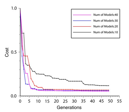
The number of models (Nm) in each subpopulation is usually an important parameter in the NGA inversion. If Nm is too small, the inversion will mainly depend on mutation operator because of poor diversity in the subpopulation, which may lead to more computational time. On the other hand, if Nm is too large, the inversion will cost much time in each generation (He et al. 2007). As a result, the total computation time is also huge although the inversion will run with fewer generations. Technically, Nm will depend on the number of variations we need to search (Sambridge and Drijkoningen 1992). Therefore, it is necessary to do some tests for different values of Nm. In this work, we do tests with some different Nm values of 10, 20, 30, and 40 (Fig. 3). Figure 3 shows, that when Nm is 10, it is clear that the convergence of inversion result is slower than other cases, which is not stable at the 50-th generation. Comparing with the result of Nm being 10, the inversion needs only about 10 generations to reach the global minima, if Nm is 30 or 40. The convergence of inversion with 20 models is a little bit slower than the case of 30 or 40 models, being stable at about the 13-th generation. Given that Nm is in proportion to the total computational time, and the inversion will cost as mentioned above, we will choose Nm to be 20 in our NGA inversion.
Figure
3.
Cost versus generations. The results are obtained with different Nms of 10 (black), 20 (red), 30 (blue), and 40 (pink)
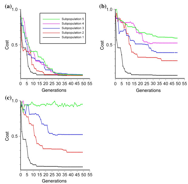
In our NGA, the most key problem is how to make subpopulations migrate into different searching niches which represent our interesting minima. This migration is controlled by the critical separation radius, Rc. If Rc is too small, then all the subpopulations will converge to the global minima, because no model is weeded out by comparison. Otherwise, if Rc is too large, all the models except those in the first subpopulation are deleted. Thus, all the subpopulations except the first one have a high Cost value and do not converge. We call these subpopulations as frustrated populations. Hence, a proper Rc is important to the number of minima we can search, especially for the number of local minima. In this study, we test the inversion with Rc of 0.1, 0.2, and 0.3. The change of Cost in the most optimal subpopulation with the generation under different Rc is showed in Fig. 4. When Rc is 0.1, all the subpopulations converge to the global minima. When Rc is 0.2, the subpopulations are separated into different niches. When Rc is 0.3, although the first three subpopulations can migrate into different minima, the fourth and fifth subpopulations become frustrated subpopulations. These results suggest that we should set Rc as 0.2 in our NGA inversion.
Figure
4.
Cost versus generations of 5 subpopulations with different Rcs of 0.1 (a), 0.2 (b), and 0.3 (c)
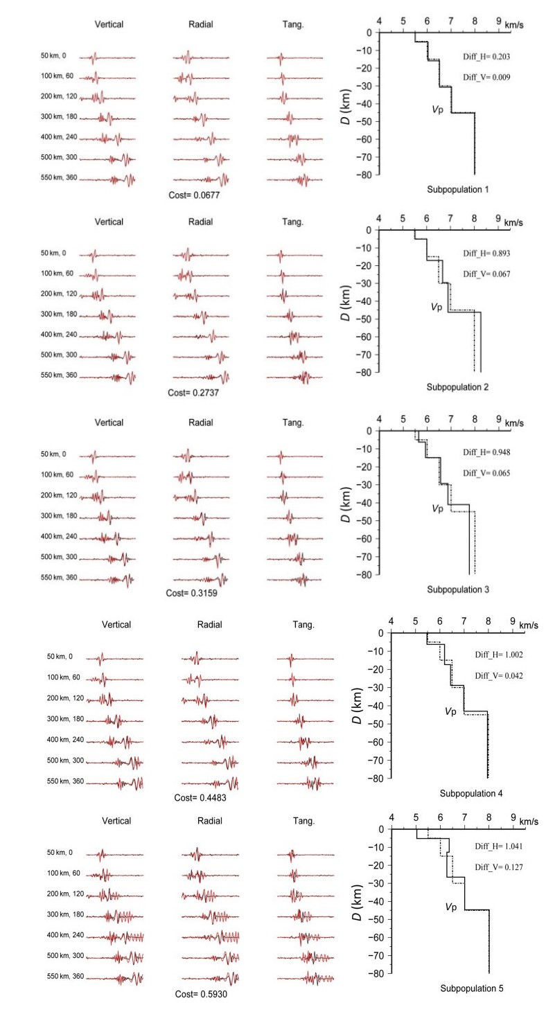
The comparison of estimated average velocity model with the SNR of 10 dB and given model in each subpopulation is presented in Fig. 5 and Table 2. The corresponding waveforms generated from these models are also shown. The first subpopulation has the lowest Cost and highest precision (the average errors are 0.009 km s-1 for velocity and is 0.203 km for thickness). Although the agreement between the true waveforms and synthetics in some subpopulations is poor, such as the waveform of 550 km distance in the 4- and 5-th subpopulations, the waveform fitness in other local minima (such as the second subpopulation) is good, which suggests multi-solutions in the NGA waveform inversion.
Figure
5.
Results from NGA inversion with unfiltered seismogram containing the SNR of 10 dB. Left Comparison of waveforms (black) generated from true model with those (red) from estimated model in the 5 subpopulations. The numbers on the left denote the distance and azimuth of the event-station pairs as shown in Fig. 1. Right Comparison of the estimated average models (solid lines) from NGA inversion with the true models (dashed lines) in 5 subpopulations. Diff_H and Diff_V indicate the average errors for thickness (in km) and velocity (in km s-1), respectively
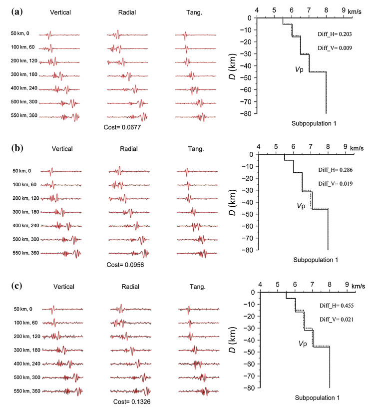
The models in the most optimal subpopulations inferred from synthetics with the SNRs of 10, 5, and 3 dB are shown in Fig. 6 and Table 3. The results of different subpopulations with the waveform containing the SNRs of 5 and 3 dB are similar as the case with the SNR of 10 dB. However, with the level of noise increasing, the accuracy of estimated models drops down. However, the biggest average errors under the circumstance of different noise are just 0.455 km for thickness and 0.021 km s-1 for velocity, which verifies the robustness of our NGA inversion for velocity structure. Besides, the biggest deviation between the true model and estimated model exists in lower crust (Fig. 6 and Table 3), which may suggest our NGA inversion have poorer constraint on lower crust comparing with other parameters. Even though, the biggest errors in lower crust are less than 1.2 km for thickness and 1.0 km s-1 for velocity, which still meets the requirement in research of 1-D crustal model.
Figure
6.
Results from NGA inversion with unfiltered seismogram containing the SNRs of (a) 10 dB, (b) 5 dB, (c) 3 dB, respectively. Left Comparison of waveforms (black) which are generated from true model with those (red) from estimated model in the most optimal subpopulation. The numbers on the left denote the distance and azimuth of the event-station pairs as shown in Fig. 1. Right Comparison of the estimated average models (solid lines) from NGA inversion with the true models (dashed lines) in most optimal subpopulation. Diff_H and Diff_V indicate the average errors for thickness (in km) and velocity (in km s-1), respectively
Table
3.
Comparison between given model and models inferred in the most optimal subpopulations with filtered and unfiltered waveforms containing the SNRs of 3, 5, and 10 dB, respectively
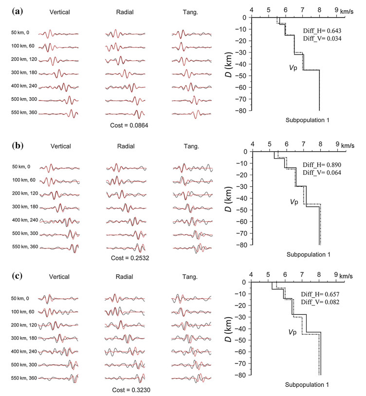
Because the true velocity structure is much more complicated than our present 1-D velocity model, the effects of lateral variations, anisotropy, and thin layer will make high-frequency wave hard to be simulated. On the other hand, the wave of high-frequency is easy to be influenced by noise in virtue of the small energy. Hence, instead of using full waveform, middle, and low frequency wave is widely used in waveform inversion. In this paper, we carry out the NGA inversion with the surface wave. First, the synthetic seismograms with the SNRs of 3, 5 10 dB are filtered between 0.02 and 0.1 Hz (Li et al. 2012; Bhattacharyya et al. 1999). Then, we use these filtered waveforms as input data of inversion. The comparison of waveforms and models are shown in Fig. 7 and Table 3. Here, we only present the model averaged from the 5 computations in the most optimal subpopulation. Comparing with Fig. 6, the model inverted from filtered wave is little worse than that of full waveform. This discrepancy embodies clearly in the velocity of sediment and the thickness of lower crust between these two models (The biggest error is 0.25 km s-1 and 1.7 km, respectively). This suggests that the surface wave has the poor constraints on the two parameters above. However, the agreement with true model in the other parameters' inversion is still great, and the total biggest average errors are only 0.675 km for thickness and 0.082 km s-1 for velocity, which can meet the requirement of interpretation and other application in consideration of the large-scale nature in seismology.
Figure
7.
Results from NGA inversion with filtered seismogram containing the SNRs of (a) 10 dB, (b) 5 dB, (c) 3 dB, respectively. Left Comparison of waveforms (red) generated from true model with those (black) from estimated model in the most optimal subpopulation. The numbers on the left denote the distance and azimuth of the event-station pairs as shown in Fig. 1. Right Comparison of the estimated average model (solid line) from NGA inversion with the true model (dashed line) in the most optimal subpopulations. Diff_H and Diff_V indicate the average errors for thickness (in km) and velocity (in km s-1), respectively
In this paper, we introduce niching genetic algorithm into the waveform inversion for 1-D crustal velocity structure. After a series of numerical tests with different objective functions, the number of models in each subpopulation, critical separation radius and level of noise, we discuss the effects of those parameters in NGA on the results and illustrate the utility of our NGA in the waveform inversion of crustal structure. Our result shows that the inversion with objective function of the zero-th lag cross-correlation has a higher precision and faster convergence than those with other functions. The number of models in each subpopulation depends on the number of variations in inversion, having a significant impact on the convergence rate and computational time. The critical separation radius is used to determine the number of local minima directly, and thus it need to be defined by some tests. The waveform inversion using the surface wave has a well-constraint on crustal velocity, which can be applied in practice.
Acknowledgments
This work was partially supported by the National Natural Science Foundation of China (Nos. 41274059, 40974021 and 40774044) and Beijing Natural Scientific Foundation (Nos. 8122039 and 8092028) to J. Lei. The GMT software package distributed by Wessel and Smith (1995) was used for plotting some figures. Anonymous reviewers provided many constructive comments and suggestions, which improved our manuscript.
Begnaud ML, McNally KC, Stakes DS, Gallardo VA (2000) A crustal velocity model for locating earthquakes in Monterey Bay, California. Bull Seismol Soc Am 90(6):1391-1408 doi: 10.1785/0120000016
Berteussen KA (1977) Moho depth determinations based on spectral-ratio analysis of NORSAR long-period P waves. Phys Earth Planet Inter 15(1):13-27 doi: 10.1016/0031-9201(77)90006-1
Bhattacharyya J, Sheehan AF, Tiampo K, Rundle J (1999) Using a genetic algorithm to model broadband regional waveforms for crustal structure in the western United States. Bull Seismol Soc Am 89(1):202-214 http://hdl.handle.net/2060/19990071219
Bina CR (1998) Free energy minimization by simulated annealing with applications to lithospheric slabs and mantle plumes. Geodyn Lithosph Earth's Mantle 1998:605-618 doi: 10.1007/978-3-0348-8777-9_21
De Jong KA (1975) Analysis of the behavior of a class of genetic adaptive systems. Ph. D. Dissertation, University of Michigan
Du ZJ, Panza GF (1999) Amplitude and phase differentiation of synthetic seismograms: a must for waveform inversion at regional scale. Geophys J Int 136(1):83-98 doi: 10.1046/j.1365-246X.1999.00711.x
Goldberg DE (1989) Genetic algorithms in search, optimization, and machine learning, ISBN: 0-201-15767-5
Goldberg DE, Richardson J (1987) Genetic algorithms with sharing for multimodal function optimization. Genetic algorithms and their applications: proceedings of the second international conference on genetic algorithms, pp 41-49
Holland JH (1975) Adaptation in natural and artificial systems: an introductory analysis with applications to biology, control, and artificial intelligence. U Michigan Press, Ann Arbor, IL
Lei JS (2011) Seismic tomographic imaging of the crust and upper mantle under the central and western Tien Shan orogenic belt. J Geophys Res 116:B09305. doi: 10.1029/2010JB008000
Lei JS (2012) Upper-mantle tomography and dynamics beneath the North China Craton. J Geophys Res 117:B06313. doi: 10.1029/2012JB009212
Lei JS, Zhao DP, Su YJ (2009) Insight into the origin of the Tengchong intraplate volcano and seismotectonics in southwest China from local and teleseismic data. J Geophys Res 114:B05302. doi: 10.1029/2008JB005881
Lei JS, Zhang GW, Xie FR (2014) The 20 April 2013 Lushan, Sichuan, mainshock, and its aftershock sequence: tectonic implications. Earthq Sci 27(1):15-25 doi: 10.1007/s11589-013-0045-9
Li HY, Michelini A, Zhu L, Spada M (2007) Crustal velocity structure in Italy from analysis of regional seismic waveforms. Bull Seismol Soc Am 97(6):2024-2039 doi: 10.1785/0120070071
Li YH, Wu QJ, Zhang R, Tiab XB, Zeng RS (2008) The crust and upper mantle structure beneath Yunnan from joint inversion of receiver functions and Rayleigh wave dispersion data. Phys Earth Planet Inter 170(1):134-146 http://or.nsfc.gov.cn/handle/00001903-5/48722
Li SH, Wang YB, Liang ZB, He SL, Zeng WH (2012) Crustal structure in southeastern Gansu from regional seismic waveform inversion. Chin J Geophys 55(4):1186-1197. doi: 10.6038/j.issn.0001-5733.04.015 (in Chinese with English abstract)
Mahfound SW (1995) Niching methods for genetic algorithms. Ph. D. Dissertation, University of Illinois, Urbana
Maurice R, Stacey D, Wiens DA, Koper KD, Vera E (2003) Crustal and upper mantle structure of southernmost South America inferred from regional waveform inversion. J Geophys Res (1978-2012) 108(B1):2038-2048 doi: 10.1029/2002JB001828/abstract
Mellman GR (1980) A method of body-wave waveform inversion for the determination of earth structure. Geophys J R Astron Soc 62(3):481-504 doi: 10.1111/gji.1980.62.issue-3
Mishra OP, Zhao DP (2003) Crack density, saturation rate and porosity at the 2001 Bhuj, India, earthquake hypocenter: a fluid-driven earthquake? Earth Planet Sci Lett 212:393-405 doi: 10.1016/S0012-821X(03)00285-1
Rodgers AJ, Schwartz SY (1998) Lithospheric structure of the Qiangtang Terrane, northern Tibetan Plateau, from complete regional waveform modeling: evidence for partial melt. J Geophys Res (1978-2012) 103(B4):7137-7152 doi: 10.1029/97JB03535
Sambridge M, Drijkoningen G (1992) Genetic algorithms in seismic waveform inversion. Geophys J Int 109(2):323-342 doi: 10.1111/gji.1992.109.issue-2
Stoffa PL, Sen MK (1991) Nonlinear multi-parameter optimization using genetic algorithms: inversion of plane-wave seismograms. Geophysics 56:1794-1810 doi: 10.1190/1.1442992
Wang Y (2014) Seismic ray tracing in anisotropic media: a modified Newton algorithm for solving highly nonlinear systems. Geophysics 79:T1-T7 doi: 10.1190/2014-0331-TIOGEO.1
Wang FY, Zhang XK (2006) Genetic algorithm in seismic waveform inversion and its application in deep seismic sounding data interpretation. Acta Seismol Sin 28(2):158-166 (in Chinese with English abstract) http://www.cqvip.com/QK/86256X/200602/21776654.html
Zhu L, Rivera LA (2002) A note on the dynamic and static displacements from a point source in multilayered media. Geophys J Int 148(3):619-627 doi: 10.1046/j.1365-246X.2002.01610.x
Table
3.
Comparison between given model and models inferred in the most optimal subpopulations with filtered and unfiltered waveforms containing the SNRs of 3, 5, and 10 dB, respectively


 DownLoad: