2024 JCR Q1
X
Advanced Search
Dai Wang, Zhuobin Wei, Jianwen Liang (2011). Response of underground pipeline through fault fracture zone to random ground motion. Earthq Sci 24(4): 351-363. DOI: 10.1007/s11589-011-0798-y
Citation: Dai Wang, Zhuobin Wei, Jianwen Liang (2011). Response of underground pipeline through fault fracture zone to random ground motion. Earthq Sci 24(4): 351-363. DOI: 10.1007/s11589-011-0798-y

Response of underground pipeline through fault fracture zone to random ground motion

More Information
  • Corresponding author:

    Jianwen Liang, e-mail: liang@tju.edu.cn

  • Received Date: 05 Jul 2011
  • Accepted Date: 13 Jul 2011
  • Available Online: 30 May 2022
  • Published Date: 09 Aug 2011
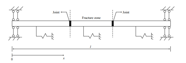
  • It is assumed that a pipeline is laid through a vertical fault fracture zone, and is excited by seismic ground motion modelled as stationary stochastic process. For horizontal incidence of waves, the cross-PSD (Power Spectral Density) function is developed using wave propagation theory, while for vertical incidence of waves the cross-PSD function is composed by auto-PSD model, coherence model and site response model. As the seismic input, the cross-PSD function is used to calculate the the axial and lateral seismic responses of underground pipeline through the fracture zone. The results show that the incident directions of seismic waves, width and soil property of the fracture zone have great influence on underground pipeline. It is suggested that the flexible joints with appropriate stiffness should be added into the pipeline near the interfaces between the fracture zone and the surrounded media.

  • The strong ground motion observations indicate that, affected by the epicenter, transmission and local site conditions, the variation of seismic ground motion with time and space is quite obviously random, so many researchers have studied the response of underground continuous pipeline in the homogeneous soil site to random ground motion (; ; ; ); however, the researches on the response of underground pipeline in heterogeneous soil site to random ground motion are not found up to now.

    In general, it is inevitable for underground longdistance pipeline to pass through the non-causative fault fracture zone, which can be regarded as one of the heterogeneous soil sites. Due to the local amplification of seismic ground motions near the fault fracture zone, underground pipeline is quite prone to be damaged, especially when the fault fracture zone is very narrow, the amplification could be very large (; , , ); therefore, it is significant for both theory and engineering to investigate the response of underground pipeline through fault fracture zone to random ground motion.

    In this paper, considering the complexity of the distribution of seismic ground motions near the fault fracture zone, the seismic response of underground continuous pipeline is studied only for two special cases, i.e., horizontal and vertical incidence of seismic waves, respectively. In addition, the observation of seismic ground motions has confirmed that the inertia force can be ignored; hence only the pseudo-static responses of underground pipeline are calculated.

    The model is shown in Figure 1; the small black blocks denote joints which are regarded as very short pipes; the pipe rests on elastic foundations and its end supports allow a rigid body motion in the axial direction.

    Figure 1. Structural model for axial motion.
    Figure  1.  Structural model for axial motion.

    If ua(x, t) denotes the absolute displacement in the axial direction as a function of the coordinate along the axis of the pipeline, and uag(x, t) denotes the ground motion, after removing the dynamic terms from the equation of axial motion of the pipe (), the pseudo-static equation can be obtained as follows

    (1)

    where ka is the soil axial stiffness per unit length; E and A are the elastic modulus and cross sectional area of the pipe or joint, respectively.

    To obtain the special solution of equation (1), ua(x, t) and uag(x, t) will be expanded over [0, l] into Fourier cosine series in the axial direction, respectively, and by means of the linear interpolation, the continuous ground motion along the pipeline at any time can be approximately replaced by the motions at discrete ground stations. The special solution plus the homogeneous solution determine the general solution

    (2)

    where B1 and B2 are undetermined constants; the elements of the matrix F are provided by ; and

    (3)

    (4)

    (5)

    (6)

    (7)

    (8)

    where xk(k=1, 2, …, m) are the axial coordinates of m ground stations with equal discrete space Δx.

    The response of the pipeline near the fracture zone is not affected by the boundary conditions when the length l is large enough; therefore, without loss of generality, the boundary conditions in Figure 1 are adopted and expressed as

    (9)

    The compatibility conditions at the interfaces between the fracture zone and the surrounded media or between the pipe and the joint are as follows,

    (10a)

    (10b)

    where xc is the coordinate at the interface; ELAL and ERAR are the axial stiffness of the left pipe or joint and the right pipe or joint, respectively; uaL and uaR are the axial pseudo-static displacements of the left pipe or joint and the right pipe or joint, respectively.

    Substituting both the boundary conditions and the compatibility conditions results in the system with 14 equations between the undetermined constants, and solving the system and substituting the obtained constants into equation (2) lead to the axial pseudo-static displacement of the pipe

    (11)

    where c is the transfer matrix of order 1×m from seismic ground motion to pipeline response.

    The pipeline response is calculated using both wave propagation theory and random vibration theory for the horizontal incidence of seismic waves, and using the pseudo-excitation method in random vibration theory for the vertical incidence of seismic waves. By using the pseudo-excitation method (), the ground pseudo-acceleration is written as

    (12)

    where L is the lower triangular matrix and satisfies the equation

    (13)

    where S is the cross-PSD function matrix of ground accelerations; "*" denotes complex conjugate; "T" denotes transpose; and eiwt is the time factor.

    Then the ground pseudo-displacement becomes

    (14)

    Substituting equation (14) into equation (11) leads to the axial pseudo-static pseudo-displacement of the pipe

    (15)

    Then the auto-PSD (Power Spectral Density) function of the pseudo-static displacement of the pipe can be expressed as

    (16)

    and the variance of the pseudo-static displacement of the pipe becomes

    (17)

    The variance of the other physical quantities such as strain etc. can be obtained in the similar way.

    The response in the direction perpendicular to the pipeline axis can be evaluated with the model shown in Figure 2; the pipe rests on elastic foundations and its end conditions allow a rigid body motion in the transverse direction.

    Figure 2. Structural model for lateral motion.
    Figure  2.  Structural model for lateral motion.

    If ub(x, t) denotes the absolute displacement in the lateral direction as a function of the coordinate along the axis of the pipeline, and ubg(x, t) is the ground motion, after removing the dynamic terms in the equation of lateral motion of the pipe (), the pseudo-static equation can be obtained as follows,

    (18)

    where kb is the soil lateral stiffness per unit length; I is the inertia moment of cross section of the pipe or joint.

    Analogous to solving equation (1), the general solution of equation (18) is

    (19)

    where D1, D2, D3 and D4 are undetermined constants and

    (20)

    (21)

    (22)

    (23)

    The boundary conditions in Figure 2 are as follows

    (24a)

    (24b)

    The compatibility conditions at the interfaces between the fracture zone and the surrounded media or between the joint and the pipe are as follows

    (25a)

    (25b)

    (25c)

    (25d)

    where xc is the coordinate at the interface; ELIL and ERIR are the bending stiffness of the left pipe or joint and the right pipe or joint, respectively; uLb and uRb are the lateral pseudo-static displacements of the left pipe or joint and the right pipe or joint, respectively.

    Using both the boundary conditions and the compatibility conditions leads to the system with 28 equations between the undetermined constants, and solving the system and substituting the constants into equation (18) result in the lateral pseudo-static displacement of the pipe. Due to the similarity of the derivations of the lateral response to the axial one by the pseudoexcitation method, the detail is omitted here.

    For the horizontal incidence of seismic waves, Figure 3 displays the schematic diagram of the fault site, which is composed of the vertical fracture zone and the surrounded media (harder than the fracture zone), and the interfaces between the fracture zone and the surrounded media are perpendicular to the pipeline axis. Seismic ground motions are evaluated as follows: first of all, suppose that the stationary stochastic process at the ground station x=0 is known; a plane wave travels along the pipeline axis with the dilatational or distortional wave velocity of soil, and the multiple reflections and refractions of the plane wave at the interfaces lead to the superposition of waves in the fracture zone; the random fields are generated by wave propagation theory (), and the cross-PSD at two ground stations is obtained by the Wiener-Khinchin formula.

    Figure 3. Fault site model for horizontal incidence of waves.
    Figure  3.  Fault site model for horizontal incidence of waves.

    In the text, suppose that the stationary stochastic process at the ground station x=0 is as follows

    (26)

    where the amplitudes A(ωk)(k=1, 2, …, n) are determined by the auto-PSD; ωk=ω1+(k-1)Δω are n discrete frequency points with equal space Δω; and φk are random phase angles of statistically independent of each other, uniformly distributed over [0, 2π].

    For the vertical incidence of seismic waves, Figure 4 shows the schematic diagram of the fault site, which is composed of the bedrock and the single soil layer with the vertical fracture zone and the surrounded media (harder than the fracture zone). Suppose that both the energy in the fracture zone and the one in the surrounded media are independent of each other; the crossPSD function is composed of auto-PSD model, coherence model and site response model, and the pipeline response is calculated by the pseudo-excitation method.

    Figure 4. Fault site model for vertical incidence of waves.
    Figure  4.  Fault site model for vertical incidence of waves.

    It is necessary to mention that absence of the statistical analysis of seismic ground motions in heterogeneous sites makes it difficult to explain exactly the variation of the parameters of auto-PSD model with ground stations near the fracture zone, so it is assumed that the parameters of auto-PSD model for the fracture zone or the surrounded media are identical to the ones of auto-PSD model for homogeneous site, respectively, and the choice of the parameters at the interfaces are made as follows. Because of using the linear interpolation among the discrete ground stations with equal space instead of the continuous ones, it is always realizable that the interfaces stand in the mid-points of the adjacent discrete ground stations for the symmetry of the pipeline response.

    In the following calculation, the auto-PSD model for ground accelerations given by is adopted and expressed as

    (27)

    where S0 is the amplitude of the white-noise bedrock acceleration; ωg and ωf are the resonant frequencies of the first filter and the second one, respectively; ξg and ξf are the damping ratios of the first filter and the second one, respectively.

    Referring to the parameters of the auto-PSD model for different soil conditions proposed by , the auto-PSD model parameters for both the fracture zone and the surrounded media are shown in Table 1. The intensity parameter S0 is chosen such that the standard deviation of the ground acceleration σa is 0.08g (g=9.8 m/s2), which corresponds to a peak ground acceleration of about 0.24g.

    Table  1.  The parameters of auto-PSD model for sites
     | Show Table
    DownLoad: CSV

    For the horizontal incidence of seismic waves, the parameters of the auto-PSD model for the surrounded media are chosen to determine the amplitudes in equation (26).

    For the vertical incidence of seismic waves, the shear-wave velocity of the single soil layer is

    (28)

    where H is the thickness of the single soil layer.

    Based on the study of a number of earthquake events recorded by the SMART-1 array, the LSST array etc., proposed a coherence model that accounts for the coherence effect,

    (29)

    where

    the model parameters are a1=0.167 8 × 10⁻⁴, a2=0.121 9 × 10⁻², b1=-0.005 5, b2=0.767 4.

    An analytical model that accounts for the site response effect due to the differences in the local soil conditions was given by

    (30)

    where

    where ωm and ξm are the resonant frequency and damping ratio of the single soil layer, respectively.

    The following parameters or notations are used in the specific numerical analysis.

    Outer radius of pipe (or joint): R=1.0 m

    Thickness of pipe (or joint): tp=0.15R

    Elastic modulus of pipe: Ep=2.07 × 10¹⁰ N/m2

    Axial stiffness of pipe: EpAp

    Bending stiffness of pipe: EpIp

    Length of joint: 0.2 m (variable)

    Axial stiffness of joint: EjAj

    Bending stiffness of joint: EjIj

    Density of soil: ρ=1.6 × 10³ kg/m3

    Poisson's ratio of soil: ν=0.25

    Shear-wave velocity of soil: vS

    Shear modulus of soil: G

    Axial stiffness of soil: ka=2G

    Lateral stiffness of soil: kb=3G

    To eliminate the effect of the boundaries on the stresses of the pipeline near the fracture zone, the pipeline length l should be large enough.

    Figure 5 shows the effect of the boundaries on the RMS (Root Mean Square) stresses of the pipeline near the fracture zone. For the vertical incidence of seismic waves (Figures 5d and 5e), the stress distribution along the pipeline only near the left interface is displayed due to the symmetry of the pipeline response. It can be seen that when the pipeline is long enough, the stresses near the fracture zone are hardly affected by the boundaries. In the following analysis, the pipe length l=400 m for axial motion and l=150 m for lateral motion are adopted, respectively; and by the tentative calculation, the equal discrete space Δx=1 m for axial motion and Δx=0.2 m for lateral motion are chosen respectively for accuracy.

    Figure 5. Effect of the boundaries on the stresses of the pipeline near the fracture zone.
    Figure  5.  Effect of the boundaries on the stresses of the pipeline near the fracture zone.

    Figure 6 shows the effect of the width of fracture zone on the RMS stresses of the pipeline without joints for the horizontal incidence of seismic waves. It can be seen that with the increase of the width of fracture zone, the peak axial stress increases beforehand and decreases afterward and always appears in the pipeline in the fracture zone, the peak bending normal stress with the similar trend to the peak axial stress is found in the pipeline in the surrounded media close to the interfaces, and the peak bending shear stress decreases gradually and appears in the pipeline in the fracture zone for the narrow fracture zone and in the surrounded media near the interfaces for the wide one, which are mainly caused by the change of phase differences of the superposed waves and the reduction of the effects of the surrounded media on both sides of the fracture zone on the pipeline in the fracture zone and on each other.

    Figure 6. Effect of the width of fracture zone on pipeline stresses.
    Figure  6.  Effect of the width of fracture zone on pipeline stresses.

    In addition, it is found that the peak axial stress is larger when the width of fracture zone is 40 m, and the peak bending stress, especially the peak shear stress, is larger when the width of fracture zone is 4 m, therefore, without loss of generality, in the following analysis of the effect of soil property on pipeline responses, the width of fracture zone 40 m for the axial responses and 4 m for the lateral ones are chosen respectively.

    Figures 7 and 8 show the effects of the soil properties of both the surrounded media and the fracture zone on the RMS stresses of the pipeline without joints for the horizontal incidence of seismic waves, respectively. It can be seen from Figure 7 that the firmer the surrounded media, the larger the peak stress, the reason for which may be that the characteristic impedance of the surrounded media is larger than the one of the fracture zone, and the reflected and refracted waves in the fracture zone are superposed in phase; the larger impedance results in the larger reflection coefficient and the smaller refraction coefficient, which means that the differences between the ground motions in the fracture zone and the ones in the surrounded media become larger. With the same explanation, the softer the fracture zone, the larger the peak stress.

    Figure 7. Effect of the property of surrounded media on pipeline stresses.
    Figure  7.  Effect of the property of surrounded media on pipeline stresses.
    Figure 8. Effect of the property of fracture zone on pipeline stresses.
    Figure  8.  Effect of the property of fracture zone on pipeline stresses.

    Figures 9 and 10 show the effect of the flexible joint on the RMS axial stresses of the pipeline for the horizontal incidence of seismic waves for the width of fracture zone 4 m and 40 m respectively. It can be found that adding the flexible joints into the pipeline near the interfaces or into the middle of the pipeline in the fracture zone can reduce effectively the peak axial stress, and the softer the joints, the more effective the reduction; In addition, if the flexible joint is added into the middle of the pipeline in the fracture zone, the location corresponding to the peak axial stress will move.

    Figure 9. Effect of flexible joints on axial stresses (W=4 m).
    Figure  9.  Effect of flexible joints on axial stresses (W=4 m).
    Figure 10. Effect of flexible joints on axial stresses (W=40 m).
    Figure  10.  Effect of flexible joints on axial stresses (W=40 m).

    Figures 11 and 12 show the effect of the flexible joint on the RMS bending stresses of the pipeline for the horizontal incidence of seismic waves for the width of fracture zone 4 m and 40 m, respectively. It can be seen that adding the flexible joint into the middle of the pipeline in the fracture zone has little influence on the peak bending stress and even leads to the amplification of the peak bending stress in the individual locations, and adding the flexible joints into the pipeline near the interfaces can reduce effectively the peak bending stress, and the softer the joints, the more effective the reduction.

    Figure 11. Effect of flexible joints on bending stresses (W=4 m).
    Figure  11.  Effect of flexible joints on bending stresses (W=4 m).
    Figure 12. Effect of flexible joints on bending stresses (W=40 m).
    Figure  12.  Effect of flexible joints on bending stresses (W=40 m).

    Figure 13 shows the effect of the width of fracture zone on the RMS bending stresses of the pipeline without joints for the vertical incidence of seismic waves. In virtue of the symmetry of the pipeline response, the stress distribution along the pipeline only near the single interface is displayed. It can be seen that with the increase of the width of fracture zone, the peak bending normal stress increases beforehand and decreases afterward, and the location corresponding to the peak bending normal stress moves from the middle part of the fracture zone to the surrounded media near the interface; and the peak bending shear stress with the similar trend to the peak bending normal stress always appears in the pipeline in the surrounded media close to the interface. The change of the peak stress may be caused by the reduction of the effects of the surrounded media on both sides of the fracture zone on the pipeline in the fracture zone and on each other.

    Figure 13. Effect of the width of fracture zone on bending stresses.
    Figure  13.  Effect of the width of fracture zone on bending stresses.

    Figure 14 shows the effect of the thickness of the single soil layer on the RMS bending stresses of the pipeline without joints for the vertical incidence of seismic waves. It can be seen that the peak bending stresses increase gradually with the increase of the thickness of the single soil layer, the reason for which is that the shear-wave velocities of both the fracture zone and the surrounded media increase with the increase of the thickness of the single soil layer, but the fracture zone compared with the surrounded media becomes softer and softer, which leads to the relative relax of the restriction of the fracture zone to the pipeline.

    Figure 14. Effect of the thickness of single soil layer on bending stresses.
    Figure  14.  Effect of the thickness of single soil layer on bending stresses.

    Without loss of generality, the thickness of the single soil layer 40 m is chosen for the following analysis of the pipeline response.

    Figures 15 and 16 show the effect of the flexible joint on the RMS bending stresses of the pipeline for the vertical incidence of seismic waves for the width of the fracture zone 4 m and 40 m respectively. It can be found that the peak bending stress can be reduced effectively for the narrow fracture zone by adding flexible joints into the pipeline in the fracture zone or the pipeline near the interfaces; and the flexible joints should be added into the pipeline near the interfaces for the wide fracture zone to reduce effectively the peak bending stress. It should be noticed that the excessively flexible joints will lead to the remarkable increase of the bending stresses of other parts of the pipeline; therefore, it is suggested that the stiffness of flexible joints should be appropriate.

    Figure 15. Effect of flexible joints on bending stresses (W=4 m).
    Figure  15.  Effect of flexible joints on bending stresses (W=4 m).
    Figure 16. Effect of flexible joints on bending stresses (W=40 m).
    Figure  16.  Effect of flexible joints on bending stresses (W=40 m).

    The seismic responses of underground pipeline through the fault fracture zone softer than the surrounded media to random ground motion are studied in this paper. The following conclusions can be drawn:

    1) The peak stress appears generally in the middle part of the pipeline in the fracture zone or in the pipeline near the interface between the fracture zone and the surrounded media, which depends on the width of the vertical fracture zone and the incidence direction of seismic waves.

    2) Compared with the surrounded media, the softer the vertical fracture zone, the larger the peak stress, which means that the underground pipeline is more prone to be damaged, and the seismic resistance of underground pipeline is more negative.

    3) The location and stiffness of flexible joints should be arranged appropriately. It is easily judged from the numerical results that the flexible joints should be added into the pipeline near the interfaces between the fracture zone and the surrounded media. The bending stiffness of flexible joint is determined chiefly by the bending stiffness of pipeline and soil property, which needs further research.

    In this paper, the seismic responses of underground pipeline are investigated only for horizontal or vertical incidence of seismic waves, and the numerical analysis for the oblique incidence of seismic waves will be given in a separate paper.

  • Clough R W and Penzien J (1993). Dynamics of Structures. McGraw-Hill, New York
    Der Kiureghian A and Neuenhofer A (1992). Response spectrum method for multi-support seismic excitations. Earthquake Engineering and Structural Dynamics 21(8): 713-740. doi: 10.1002/(ISSN)1096-9845
    Der Kiureghian A (1996). A coherency model for spatially varying ground motions. Earthquake Engineering and Structural Dynamics 25(1): 99-111. doi: 10.1002/(ISSN)1096-9845
    Hindy A and Novak M (1980). Pipeline response to random ground motion. Journal of Engineering Mechanics 106: 339-360. https://www.researchgate.net/publication/247185040_Pipeline_response_to_random_ground_motion
    Liang J (1998). Dynamic analysis of pipelines laid through three-soil media. Journal of Tianjin University 31(2): 163-168 (in Chinese with English abstract). http://en.cnki.com.cn/Article_en/CJFDTOTAL-TJDX802.005.htm
    Liang J, Feng L and Ba Z (2009). Scattering of plane SV waves by local fault site. Journal of Natural Disasters 18(5): 94-106 (in Chinese with English abstract) http://en.cnki.com.cn/Article_en/CJFDTOTAL-ZRZH200905014.htm
    Liang J, Feng L and Ba Z (2010). Amplification of plane SH waves by a local fault with fracture zone. Acta Seismologica Sinica 32(3): 300-309 (in Chinese with English abstract). http://www.en.cnki.com.cn/Article_en/CJFDTOTAL-DZXB201003006.htm
    Liang J, Feng L and Ba Z (2011). Diffraction of plane P waves around a local fault. Rock and Soil Mechanics 32(1): 244-252 (in Chinese with English abstract). https://www.researchgate.net/publication/290288848_Diffraction_of_plane_P_waves_around_a_local_fault
    Lin J H and Zhang Y H (2004). Pseudo-Excitation Method for Random Vibration. Science Press, Beijing, (in Chinese).
    Qu T, Wang J and Wang Q (1996). A practical model for the power spectrum of spatially variant ground motion. Acta Seismologica Sinica 18(1): 55-62 (in Chinese with English abstract). http://adsabs.harvard.edu/abs/1996AcSSn...9...69Q
    Ren C and Luo Q F (2005). Effect of fault fracture zone on the ground motion of non-causative fault site. Journal of Seismological Research 28(2): 162-166 (in Chinese with English abstract). http://en.cnki.com.cn/article_en/cjfdtotal-dzyj200502010.htm
    Shuai J, Lv Y M and Cai Q K (1999). Stationary random vibrations of buried pipelines. Journal of the University of Petroleum 23(4): 65-70 (in Chinese with English abstract). https://www.researchgate.net/publication/295375524_Stationary_random_vibrations_of_buried_pipelines
    Wang D, Qu T and Liang J (2010). Effect of spatial coherence of seismic ground motions on underground continuous pipeline. Journal of Vibration Engineering 23(2): 145-150 (in Chinese with English abstract). http://en.cnki.com.cn/Article_en/CJFDTOTAL-ZDGC201002004.htm
    Zerva A, Ang A S H and Wen Y K (1988). Lifeline response to spatially variable ground motion. Earthquake Engineering and Structural Dynamics 16(3): 361-379. doi: 10.1002/(ISSN)1096-9845
  • Related Articles

Catalog

    Corresponding author: Jianwen Liang, liang@tju.edu.cn

    1. On this Site
    2. On Google Scholar
    3. On PubMed

    Figures(16)  /  Tables(1)

    Article views (393) PDF downloads (3) Cited by()

    /

    DownLoad:  Full-Size Img  PowerPoint
    Return
    Return
    x Close Forever Close