Benchmark on the accuracy and efficiency of several neural network based phase pickers using datasets from China Seismic Network

1.   Introduction

Picking seismic phases is the most fundamental and critical task in seismological studies. Identifying signals traveling along different ray paths and picking their onset times are the basic and crucial tasks for earthquake detection, travel-time tomography and many other studies. Seismic records and dense array observations provide abundant and continuous data; as a result, efficient automatic phase pickers have been extensively used to process large datasets. The recent development of seismic pickers based on deep learning neural networks (DNN) has provided unique advantages. Many state-of-the-art DNN models have been developed and applied (Ross et al., 2019; Zhu WQ and Beroza, 2019; Mousavi et al., 2020; Soto and Schurr, 2021; see also Bergen et al., 2019; Kong QK et al., 2019). These models can take advantage of large, labeled datasets and thus outperform traditional picking methods in certain scenarios.

Most seismic pickers originate from computer vison (CV) and natural language processing (NLP) because the three components of seismic records are analogous to the RGB image channels and are time series, similar to the audio and text processed via NLP. Moreover, seismic phases are routinely picked by analyzers, thus an abundance of labeled data are available for model training. Well-developed network CV and NLP structures could be easily implemented by seismologists, which has led to the rapid development of DNN seismic pickers.

The most widely used basic network structures are the convolutional neural network (CNN), recurrent neural network (RNN), and Transformer (Hochreiter and Schmidhuber, 1997; LeCun et al., 1998; Vaswani et al., 2017). Some early pickers employed a basic CNN model (Ross et al., 2018). Subsequently, a simple recurrent network model for object symmetry detection (Ke W et al., 2017) was used to pick P/S phases (Wang J et al., 2019). UNet is a CNN that was developed for biomedical image segmentation (Ronneberger et al., 2015) and has been coopted by seismologists to produce the most popular DNN picker, PhaseNet (Zhu LJ and Beroza, 2019). UNet++, the successor of UNet, has also been used to improve the performance of seismic models (Li WW et al., 2021). Recently, Yu ZY and Wang WT (2022a) developed a lightweight phase picking network (LPPN) based on the Yolo V3 real-time object detection algorithm (Redmon and Farhadi, 2018) to process large-scale seismic data. The Transformer (Vaswani et al., 2017) has also been adopted to create the EQTransformer picker, with the aim of improving model sensitivity through attention mechanism (Mousavi et al., 2020).

Most seismic models require a CNN to process the original waveforms, while for model optimization, such as for skip-connections, a deep separable network can be utilized to improve performance. Combining a CNN and a RNN can provide greater contextual information and processing speeds (Zhou YJ et al., 2019; Hu JP et al., 2020). A generative adversarial network may also be used to reduce false P-phase triggers for early warning applications (Li ZF et al., 2018).

DNN pickers have been extensively used worldwide to identify aftershocks, map faults, and extract travel-times (Wang J et al., 2019; Jiang CX et al., 2022; Liu M et al., 2020; Wang RJ et al., 2020). They have also been widely applied in seismological studies across China. For instance, Zhu LJ et al. (2019) trained one CNN-based phase-identification classifier (CPIC) using a small training dataset containing 30,146 phases from 4,986 aftershocks following the M_W7.9 Wenchuan Earthquake. By applying CPIC to one-month of continuous recordings from 14 stations, the authors were able to detect 97.5% of the manually picked phases. Using the same dataset, Zhou YJ et al. (2019) developed a hybrid algorithm using sequenced CNN-RNN networks for earthquake detection and phase picking. Their algorithm could detect 94% of the aftershocks and the magnitude of picking error for P- and S-phases was ~0.03 s (S.D. ≈ 0.5 s). More recently, Zhou PC et al. (2021) applied the PhaseNet model, trained using a dataset from California, USA, to a temporal array deployed in Weiyuan, Sichuan. Owing to the dense array and efficient automatic processing, their event catalog contained nearly 60 times as many earthquakes as those in the manual report. Zhao M et al. (2021) similarly applied PhaseNet to 21 stations located within 75 km of M_S6.0 Changning Earthquake to identify aftershocks; transfer leaning was applied by adding 120,233 phases from 16,595 local earthquakes to re-train the original PhaseNet algorithm, which improved both the accuracy and error distribution. Hu JP et al. (2020) trained a combined CNN-RNN model to pick the P-phases of small events near the Dagangshan Reservoir in Sichuan. Their model was trained using 376,283 Pg-phase picks from 70,729 local earthquakes for which M_L=0–3 and achieved an accuracy of 90.7% with a recall of 92. 6%. Using the original PhaseNet, Su JB et al. (2021) built a rapid aftershock catalog for the M_S6.4 Yangbi Earthquake to map the underlying fault structure. The derived travel-times were subsequently used by Zhang YP et al. (2021) to reconstruct the fine-scale crustal velocity structure. Yu ZY and Wang WT (2022b) also applied a CNN picker (Yu Z et al., 2020) to the same dataset to develop the FastLink association algorithm.

The performances of DNN pickers have varied among studies because the distribution of stations, record quality, and earthquake characteristics of different regions can affect model performances. The models have also been trained using different datasets and applied to records at various distances and of different qualities. Typically, DNN models show a high precision on their own training and test datasets, while it is unclear how they may perform when applied to novel test data. Analyzing the performance of different models using a uniform dataset may allow us to objectively compare picker performance, which should in-turn drive further model improvements and assist end-users in choosing the most suitable picker for their data.

Woollam et al. (2022) developed the SeisBench framework to benchmark different models across several different datasets. While simple comparisons have been made using several aftershock sequences (Jiang C et al., 2021), such benchmarks have not been set in China. A large-scale Chinese seismic dataset, DiTing, was recently made public (Zhao M et al., 2023). It contains approximately 2.73 million three-component records sampled at 50 Hz. The earthquakes in the dataset are distributed across all Chinese mainland with magnitudes ranging from 0 to 7.7. This provides an opportunity to benchmark DNN pickers using one uniform dataset.

In this study, we compared several DNN phase pickers using the DiTing dataset. Using the PyTorch framework, we implemented the popularly used PhaseNet, EQTransformer as well as the RNN and LPPN models we have developed. The performances of these pickers, including precision, recall, and computational efficiency, were evaluated using the same training and test datasets on both CPU and GPU devices. The consistent deep learning framework, dataset, and devices ensured the fair comparison of these models and provided reference for their performances. Uniform application processing interfaces (APIs) were also designed so that developers could add more models. We also provided one tutorial and two sets of binary models trained at sampling rates of 50 Hz and 100 Hz for use by end-users.

2.   Data and methods

2.1   Dataset

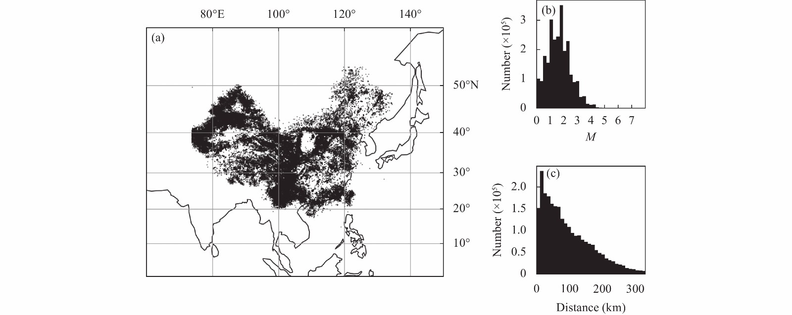
The DiTing dataset was used to benchmark several DNN pickers. This dataset was constructed from records collected by the China Seismic Network (CSN) from 2013 to 2020. Each data sample contains 180-second-long, three-component seismic waveforms with manually picked P- and S-phases. Waveforms begin at a random number of seconds before the corresponding earthquake occurrence time. The maximum epicenter-to-station distance is set to 330 km. The dataset contains 787,010 regional seismic events with magnitudes ranging from 0 to 7.7 and 2,734,748 three-component waveforms with corresponding P- and S-picks, covering most of the seismological active regions in China. The DiTing dataset offers the advantages of abundant data, high label quality, large areal coverage and favorable distances (Zhao M et al., 2023). It can thus be used in seismological artificial intelligence studies focusing on seismicity in China.

The data used in this study are illustrated in Figure 1. As the dataset does not provide the location of the earthquakes due to data policies, we used events listed in the official catalogs from 2013–2020 for which M ≥ 0 as their distributions. To evaluate picker performance, we split the total dataset into training and validation data, using 90% of all samples (approximately 2.46 million samples) for training. The remaining 0.27 million samples were used for model validation. All models shared the same training and validation data.

Figure  1.  Distributions of events (a), magnitudes (b), and epicentral distances (c) based on the DiTing dataset used for DNN picker benchmarking. The solid line is the boundary of mainland.

DownLoad: Full-Size Img PowerPoint

2.2   Seismic phase pickers

We evaluated seven phase pickers, including the most widely used DNN structures, such as CNN, RNN, Transformer, and their combinations. To ensure a fair comparison, all models were re-implemented in the PyTorch framework and some were slightly modified to allow for easy labeling and rapid convergence. The evaluated models include UNet (PhaseNet), UNet++, EQTransformer，RNN, and three LPPN models, which are briefly summarized.

PhaseNet is the most widely used DNN phase picker (Zhu WQ and Beroza, 2019; Liu M et al., 2020; Su JB et al., 2021; Zhao M et al., 2021). It is called UNet in CV and it is a modified encoder-decoder model that consists of a CNN encoder to extract features from waveforms and a CNN decoder to output classifications. Inputs and outputs have the same number of data points, forming a point-to-point phase picker. To increase accuracy, UNet adds a skip-connection between the encoder and decoder. Its successor, UNet++, adds more skip-connections for better performance (Zhou YJ et al., 2019); as a result, it is more accurate and contains a more complex internal structure than UNet (Li WW et al., 2021).

RNN is another point-to-point phase picker. It is a CNN-RNN fusion model in which the CNN and RNN layers are used to extract waveform features and to process the extracted features, respectively. Hu JP et al. (2020) used a bidirectional RNN model to extract more features from waveforms. The RNN structure has a broad receptive field, which is defined as the region in the input space at which a particular feature is looking. For seismic waveforms, the receptive field can be regarded as the length of time window from which the feature is extracted (Yu Z et al., 2020). In general, RNNs can process longer contexts and have broad receptive fields that allow for a high degree of accuracy (Hu JP et al., 2020). The RNN picker in this study was modified from EQTransformer by removing the Transformer layers.

EQTransformer is a state-of-the-art picker that utilizes both event detection and phase picking (Mousavi et al., 2020). It was constructed by combining a CNN, a RNN, and a Transformer. By adding a Transformer into an RNN model, the resulting EQTransformer has a more complex structure. As we aimed to evaluate picker performance, we removed the detection output from the original EQTransformer by exchanging three decoders for one. This modification made data labeling easier and improved model convergence speeds. The attention scheme was maintained to ensure model performance (Mousavi et al., 2020; Hu YM et al., 2021). The modified EQTransformer (hereafter, EQT) can simultaneously detect different seismic phases.

In addition to the point-to-point pickers, we analyzed the performance of LPPN models (Yu ZY and Wang WT, 2022a) that we developed to process large-scale continuous dense array records. LPPNs works via single classification and regression, extract features using a CNN, and down-sample in the extracted feature domain to broaden the receptive field. Such models produce only a single probability for N consecutive points to classify a segment as a P-/S-phase or neither. The arrival time is then obtained through regression. Both the number of features and stride N are configurable to meet different scenarios (Yu ZY and Wang WT, 2022a). In this study, we set the stride $N= 8$ and evaluated three models with different numbers of features as tiny, medium, and large models. Owing to the feature domain down-sampling scheme, LPPNs can run quickly on various devices.

2.3   Labeling scheme for model training

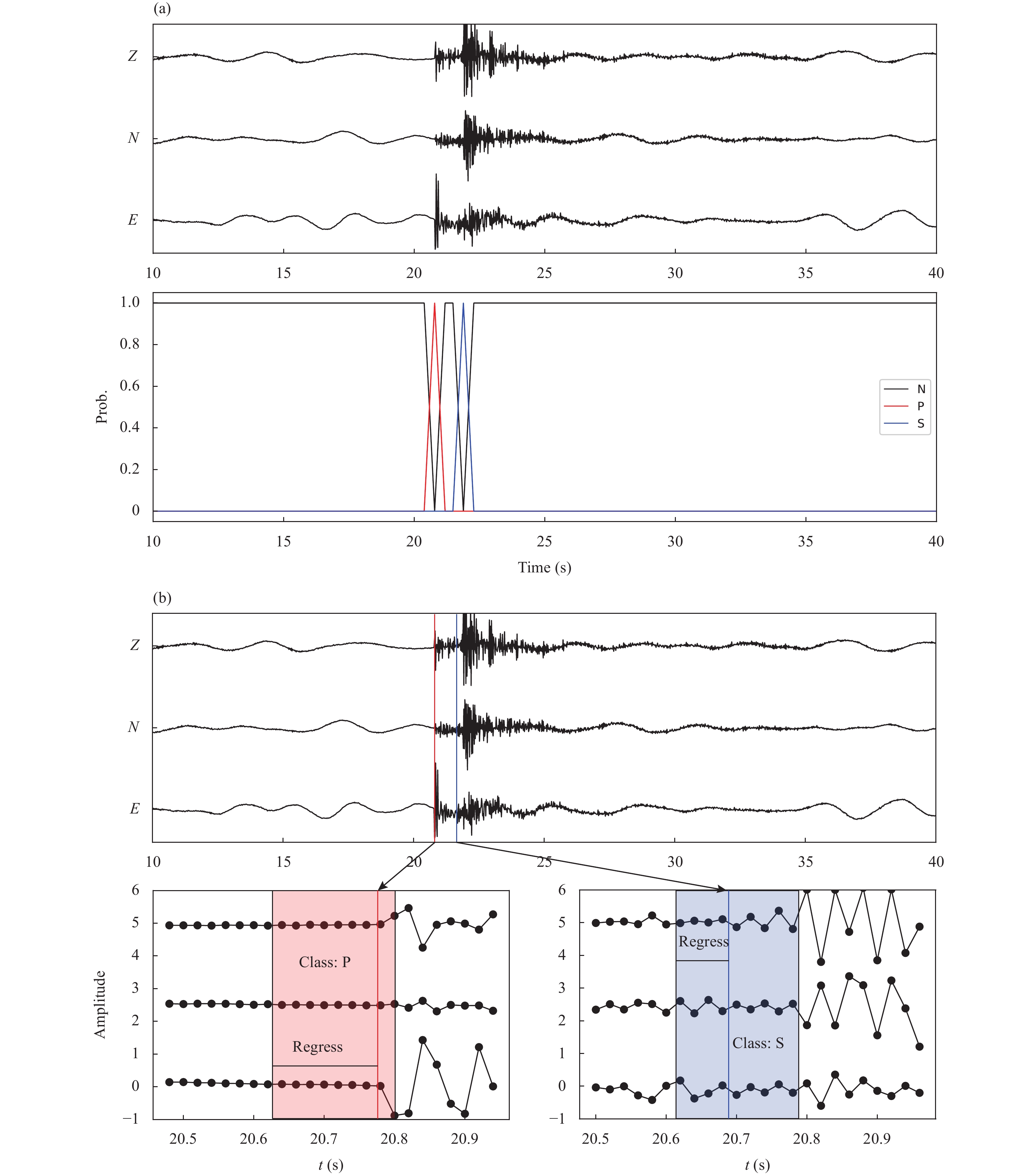
All the evaluated pickers are supervised learning and thus require labeled samples for training. When training the models, waveforms were cropped to 6,144 sampling points [ $x\in {\mathbb{R}}^{3\times 6144}]$ (122 seconds for the DiTing dataset) and P- and S-phases could be in any position of the window. All models shared the same input data, but the labels differed; we used two labeling schemes — one for the LPPN models and the other for the point-to-point models (Figure 2). UNet, UNet++, RNN, and EQT all yield point-to-point outputs, wherein each output data point contains the probability of each of the three phase types: P, S, and “none” (i.e., not P-/S-phases). The probability of a data point as the manual pick is equal to 1.0. Considering the uncertainties of manual picks, a symmetrical triangular probability window with a width of 40 sampling points (0.8 s at a sampling rate of 50 Hz) centered at the manual pick was used. The probability of “none” was ${d}_{{\rm{None}}}=1-{d}_{{\rm{P}}}-{d}_{{\rm{S}}}$, where ${d}_{{\rm{P}}},{d}_{{\rm{S}}}$ is the probability of a P- or S-phase. The triangular window was adopted from EQTransformer. We also compared the Gaussian window in PhaseNet (Zhu WQ and Beroza, 2019), which provided nearly the same result (Appendix 1).

Figure  2.  Labeling schemes used to train different pickers. (a) EQT, RNN, UNet, and UNet++; (b) LPPN models.

DownLoad: Full-Size Img PowerPoint

LPPN models require labels for phase-type classification and regression. Phase types are classified using eight consecutive points, where the classification label, ${c}_{t},$ denotes the type of the sampling points ${x}_{8t:8t+8},$ and the regression label, ${r}_{t}$, represents the location of a phase between $8t$ and $8t+8$. The entire waveform is then divided into small segments containing eight data points and the integer of the $k$-th data point, k/8, is taking as the segment index. If a data point ${x}_{k}$ is defined as the P-/S-phase arrival, the classification label, ${c}_{⌊\frac{k}{8}⌋},$ is assigned as P/S and the regression label, ${r}_{⌊\frac{k}{8}⌋}=$kmod (8) represents the number of points away from the start of the segment. If there are no P- or S-phase picks, the classification label is set to “none” and the regression label ${r}_{⌊\frac{k}{8}⌋}=0$.

2.4   Model training

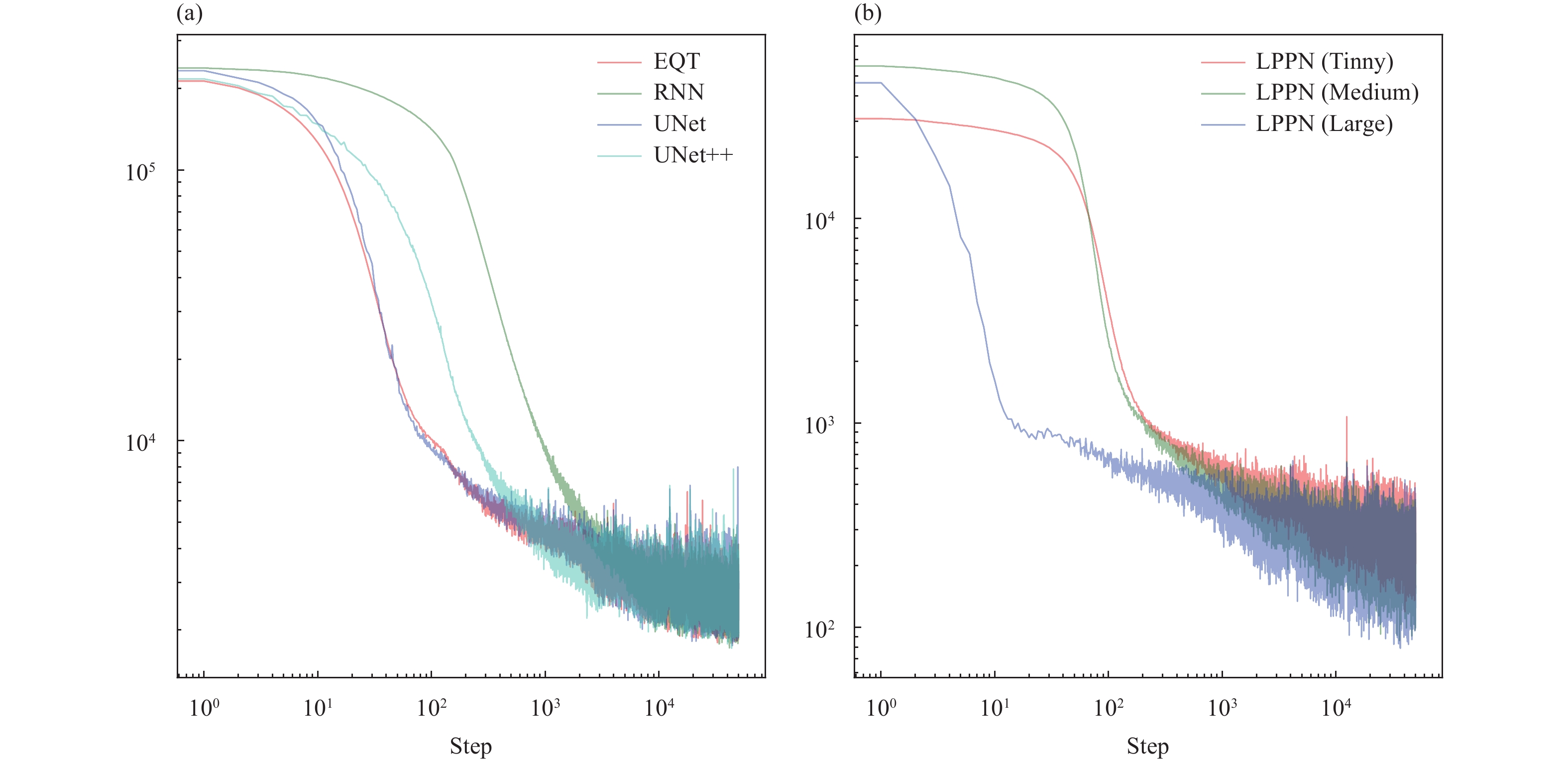
Minimal data pre-processing was conducted during the training and validation of our models. Each waveform was simply normalized using the maximum absolute value and these normalized waveforms were taken as input. The UNet, UNet++, RNN, and EQT models had the same loss functions as cross entropy (Figure 3a):

Figure  3.  Variations in the outputs of loss functions during model training for (a) EQT, RNN, UNet, and UNet++ and (b) the LPPN models.

DownLoad: Full-Size Img PowerPoint

where $T$ is the number of sampling points (6,144 in current study.) and ${p}_{i,c}$ is the probability output for the $i$-th sampling point of the $c$-th class. Meanwhile, the loss function of the LPPN models (Figure 3b) consisted of both classification (cross entropy) and regression (mean square error):

where ${p}_{i,c}$ is the probability of the $i$-th sampling point. The first expression is cross entropy loss, and the second is the mean square error loss. However, only the output of either the P- or S-segment is necessary for regression. We added the weight, ${w}_{i},$ to mask the output of “none-type” phases during regression, which was set equal to 0. Though the loss outputs of the models differed in magnitude, all models converged after 10,000 iterations.

3.   Model performance and efficiency

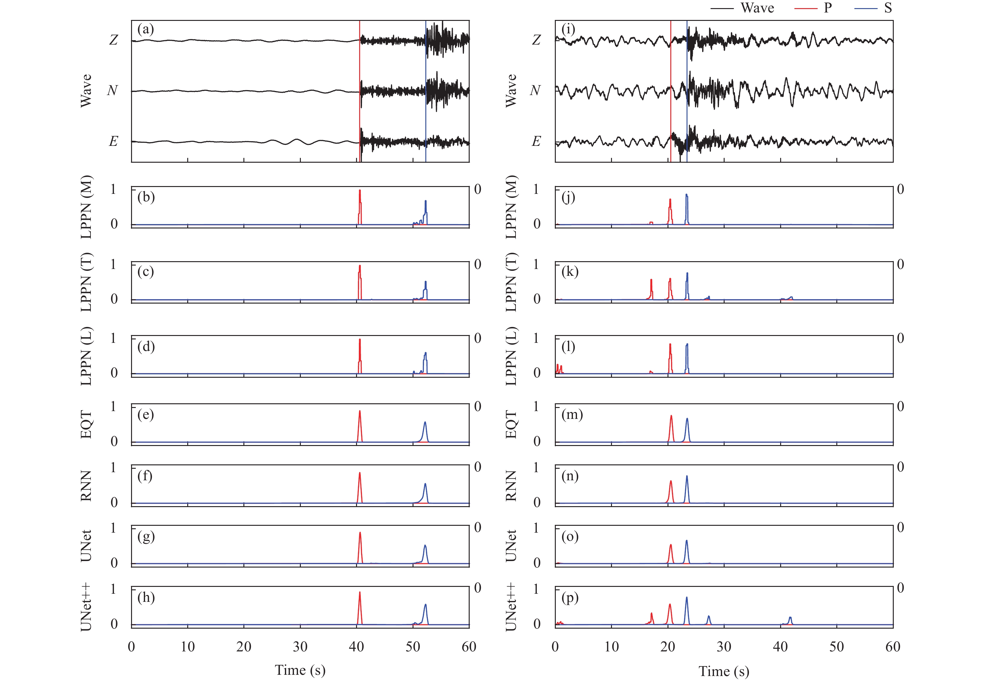
We analyzed two key features — performance and efficiency — for all seven models in this study. Figure 4 shows two examples of individual picking outputs from all the models. Two sets of three-component records were used to show the probability outputs of each model and each component had 6,144 data points with a time length of ~120 s. As shown in Figure 4, for both high- and low-signal-to-noise ratio (SNR) waveforms, all models correctly output high probabilities around the manual picks. The models could predict both the type and arrival times of corresponding P- and S-phase arrivals. The probability of an S-pick was generally lower than that of a P-pick, which agrees with the facts that S-waves are usually preceded by P codas and have more complex waveforms for picking with a high degree of confidence (Zhu WQ and Beroza, 2019). We also observed some false picks in the low-SNR waveforms, some of which were located at the edge of the time window and were likely caused by convolution, resulting in artifacts near both ends of windowed waveforms (Hu JP et al., 2020). The remaining false picks were likely due to noise in the data, which may be identified as the onset of P-/S-phases; however, their probabilities were lower than those of true P/S arrivals.

Figure  4.  Probability outputs of different models for high-SNR (a–h) and low-SNR (i–p) waveforms. The vertical red and blue solid lines over the normalized waveforms indicate the manual P- and S-picks.

DownLoad: Full-Size Img PowerPoint

Over 160,000 samples were used to comprehensively evaluate the seven models. We also constructed an ensemble learning model by simply averaging the outputs of the point-to-point models (EQT, RNN, UNet, and UNet++). The model was constructed using a bootstrap aggregation (bagging) strategy to reduce error, such that:

where ${p}_{m}$ is the probability output by model m ( $m\in \{{\rm{EQT}},{\rm{RNN}},{\rm{UNet}},{\rm{UNet}}++\}$) and the statistical standard for bagging was same among the models.

There are three types of picked samples: true positive (TP, corrected picks) samples, false positive (FP) samples and false negative (FN) samples. To address how well the models picked phases, we analyzed their precision (P) and recall (R). Precision is the fraction of TP among all picks, $P={\rm{TP}}/({\rm{TP}}+{\rm{FP}})$, and recall (R) is the fraction of TP picks among all possible picks, $R={\rm{TP}}/({\rm{TP}}+{\rm{FN}})$. The F₁-score defined as the harmonic mean of P and R, ${F_1}=2PR/(P+R)$, was used to indicate model performance. When evaluating the mean and standard deviation of picking misfit, only those picks for which misfit < 1.5 s were counted. These parameters were determined using the following rules:

1. If a probability exceeded a given threshold, it was taken as an effective pick;

2. If the misfit between the pick and the manual pick was less than 0.5 s, it was defined as a TP sample; otherwise, it was defined as an FP sample;

3. If no TP picks were found for a manual pick, the sample was defined as an FN sample.

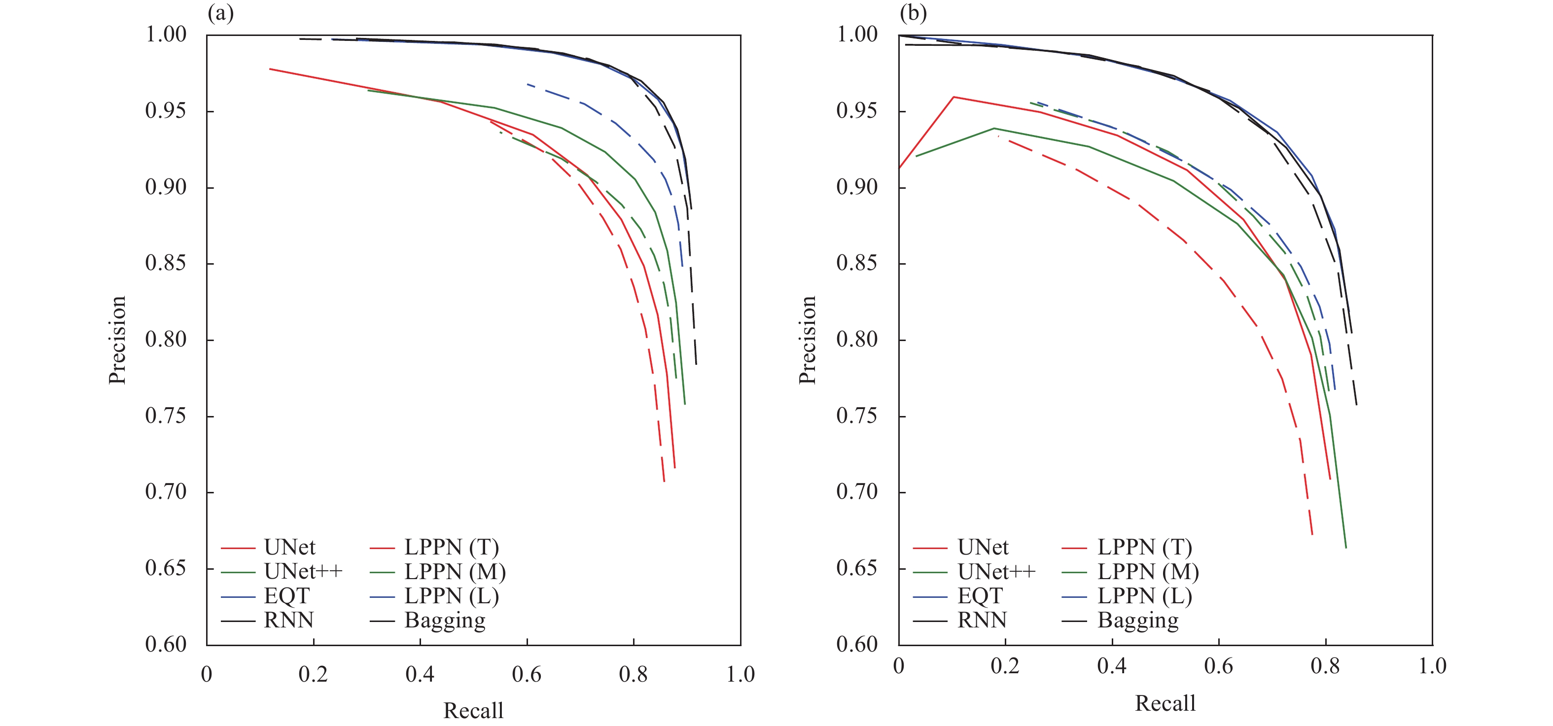
The P-R curves of the seven models and after bagging are shown in Figure 5. The P and R for P-picks were generally better than those for S-picks. Among the models, RNN and EQT exhibited similar performances and outperformed the others. With additional training parameters and model optimization, UNet++ performed better than UNet. The performances of the LPPN models depended on their sizes, with the large model performing better than UNet++, although not as well as RNN or EQT. The performance of the medium-sized model was between those of UNet and UNet++, while that of the tiny model was slightly below UNet due to the limited number of training parameters.

Figure  5.  P-R curves for the seven models and bagging. (a) P- and (b) S-picks. Abbreviations: (T): Tiny; (M): Medium; (L): Large.

DownLoad: Full-Size Img PowerPoint

Probability thresholds affect the precision, recall, and F₁-scores of models. Figure 6 shows how these parameters varied with a given threshold. As expected, when the threshold increased, recall decreased and precision increased. While each model should have its own optimal threshold, all the models we examined had high F₁-scores near a threshold of 0.3 and the curves of F₁-scores were almost flat near this value (Figure 6). For all subsequent evaluations, we selected 0.3 as the common probability threshold for all models to aid in comparison. More details are summarized in Figure 7. Taking 0.3 as the probability threshold, we calculated the P, R, and F₁-score of these models, as well as the mean and standard deviation of the misfit between the model and manual picks. These metrics generally agreed with the P-R curves, which showed that model performance was better for P- than for S-picks. Gaussian distributions of misfit indicated that the picking results were stable. The standard deviation of P-picks was less than that of S-picks; those for P-picks were less than 200 ms and those for S-picks were less than 300 ms. The means for P-picks were less than ±20 ms，equivalent to approximately one data point for the 50-Hz waveforms. The mean misfit of S-picks was slightly larger but still less than 40 ms. For P-picks, precision ranged from 0.805 (LPPN Tiny) and reached 0.943 (EQT). For S-picks, precision ranged from 0.777 (LPPN Tiny) to 0.904 (EQT). The recalls for these models exceeded 0.8 for P-picks and 0.7 for S-picks, meaning that at least 80% of the P- and 70% of the S-arrivals in the test dataset were successfully identified and correctly picked. Training using a large-scale dataset ensured the high performance of all the models.

Figure  6.  Variations in precision, recall, and F₁-score with increasing probability thresholds across all models for the P-phase (a) and S-phase (b).

DownLoad: Full-Size Img PowerPoint

Figure  7.  Statistical metrics of the seven models and bagging for P-picks (a) and S-picks (b).

DownLoad: Full-Size Img PowerPoint

Taking the F₁-score as the standard, the RNN model exhibited the best performance for both P- and S-picks. The F₁-scores for EQT were slightly lower than those for the RNN, being approximately 0.02 for P-picks and 0.004 for S-picks, indicating that these two models, with their large receptive fields, performed similarly. The remaining models had similar P-R curves, with the F₁-scores of P-picks ranging from 0.815 (LPPN Tiny) to 0.882 (LPPN Large) and those of S-picks ranging from 0.746 (LPPN Tiny) to 0.808 (LPPN Large). Although the F₁-scores for the bagging model were not the highest, both the mean and standard deviation were the lowest among the models. This was expected since averaging improves model performance in the aspect of error statistics.

The P and R values in this study were generally less than those obtained over smaller regions (Zhu WQ and Beroza, 2019; Yu ZY and Wang WT, 2022a), though some manual picks were missed, as indicated by the lower recall values. The DiTing dataset contains a vast assortment of labels from different regions and by different operators. Different picking thresholds and qualities may be one reason for the lower recall values. We calculated the number of FN, TP, and FP samples for different SNRs and grouped them using an SNR interval of 1.0. Recalls were then calculated for each interval, as shown in Figure 8. Most of the missed picks had low SNRs (< 1). While DNN approaches performed better than traditional methods at low SNRs, the SNR still affected model performance (Ross et al., 2018; Zhu WQ and Beroza, 2019).

Figure  8.  Recalls of different models with different SNRs for P-phases (a) and S-phases (b).

DownLoad: Full-Size Img PowerPoint

The number of correct picks depended on the probability threshold, which was set to 0.3, as shown in Figure 7. Increasing a threshold will typically improve the reliability of the picked phase. Nevertheless, a high probability threshold will also lead to a certain number of true phases being discarded. Based on the 160,000 test samples, we calculated the probability distribution for correct (TP) and incorrect (FP) picks for both P- and S-phases (Figure 9). The numbers of TP and FP picks were normalized by the total number of picks, where $N={\rm{TP}}+{\rm{FP}}$. It is clear that the probabilities of correct P-picks were higher than those of S-picks, indicating that it was easier to pick P-phases reliably and with a high degree of confidence. As expected, TP picks usually occurred when the probability was high for both P- and S-phases. The probability was also model dependent. The bagging model incorporated the probabilities of four models via averaging, so the TP and FP picks were more strongly correlated with probability. Because the LPPN models used only one segment (composed of eight points in this study) to pick phases, and it is easier to achieve a high probability for one phase, the rate of high probabilities for TP picks was higher than for the other models. Moreover, the EQT and RNN models produced fewer false picks, likely benefiting from their broad receptive fields, which enabled them to capture more features, resulting in improved accuracy.

Figure  9.  Probability distributions for TP and FP picks among P-picks (a) and S-picks (b). The numbers of TP and FP samples at a probability threshold of 0.3 are shown in the top left of each panel.

DownLoad: Full-Size Img PowerPoint

The mean absolute error and standard deviations of the TP picks with different probability thresholds are summarized in Figure 10. All values decreased significantly when the probability threshold increased, indicating that the picks with higher probabilities were closer to the manual picks. The statistics shown in Figures 9 and 10 may be of aid in choosing a suitable probability threshold when applying the models to real data; however, the choice is still ad-hoc and depends on the desired picking qualities. If high-quality picks are desired, such as for tomography, a high threshold is preferred, while we may miss more TP samples with a higher threshold, as shown in Figure 5. Therefore, when detecting aftershock sequences from continuous data, a lower threshold may be better because the FP picks will be further qualified and removed during phase association process. Moreover, the FP picks may also include some unlisted true phases. Because the manual picks in the DiTing dataset have been reviewed by analysts (Zhao M et al., 2023), there should be fewer unlisted phases than labeled ones and so, statistically, it can serve as a reference for end-users to choose a suitable probability threshold for their applications.

Figure  10.  Mean absolute error and standard deviation for TP picks with different thresholds. (a) Mean absolute error and (b) standard deviation for P-picks; (c) mean absolute error and (d) standard deviation for S-picks

DownLoad: Full-Size Img PowerPoint

In addition to performance, efficiency is a major concern when applying models to continuous data. The efficiency or computing cost of a model is mainly controlled by the number of parameters and the network structure, which can be represented by logical calculations estimated as giga floating point operations (GFLOPs). Using the seven trained models, excluding the bagging model, we processed three-component continuous data. For each component, there were 8,640,000 data points that corresponded to two days of records at a sampling rate of 50 Hz. Computation was performed using both CPU and GPU devices. As the models were trained with 6,144 sampling points, we cut the continuous data into 1,440 pieces, with each piece containing 6,144 sampling points. The server running the evaluation had a 32-core TR-3975WX CPU (Advanced Micro Devices, Inc., USA) and a Nvidia TITAN RTX GPU with 24 GB memory (Nvidia Corp., USA).

To test the real efficiency of the pickers on different devices, we used ONNX (https://onnx.ai; The Linux Foundation, 2019) to deploy different models (see the Supporting Materials for model generation in ONNX). The time costs are summarized in Table 1. The CNN structure was common to all of the models and used to process raw waveforms; this may be easily parallelized with a GPU. For each model, the time cost when using a GPU device was much less than when using a CPU. As the LPPN models were specially designed to improve computational speed, they contained fewer parameters than the other models (LPPN Tiny and Medium) and exhibited higher efficiencies even when more model parameters were added (LPPN Large). UNet++ required the longest run-time, which was consistent with its largest number of parameters and GFLOPS. The peak memory of UNet++ can exceed the boundaries of 24G, so the speed on a GPU was similar to that on a CPU.

Table  1.  Inferred times, GFLOPs, and numbers of parameters of different models.

Model	Inferred time (ms)		GFLOPs	No. parameters (×103)
	CPU	GPU
EQT	7091	145	100.5	423.2
RNN	6198	121	111.9	450.3
UNet	1198	82	72.9	173.2
UNet++	23021	19852	4540.6	3061.8
LPPN (T)1	351	50	12.2	11.0
LPPN (M)2	607	85	45.8	41.7
LPPN (L)3	990	132	479.4	655.2

 | Show Table

DownLoad: CSV

As can be seen from Table 1, UNet++ was the least efficient. This may be due to this model having the largest scale and demanding tremendous memory consumption. The other CNN-based models, except for UNet++, were faster than the RNN-based models on the CPU because CNN models can be more easily parallelized by a GPU to greatly increase their speeds. Although the GFLOPs of UNet was smaller than that of LPPN Large, it was slower than the LPPN on a CPU but faster on a GPU. Model structures may affect their efficiency. The differences in GFLOPs and model parameters are further illustrated in Figure 11a, b. We also summarized the F₁-scores of these models in Figure 11 to make it easier to choose a balance between efficiency and performance. P- and S-phases were picked simultaneously and had the same inferred times but different F₁-scores. The RNN and EQT models had higher F₁-scores and intermediate inferred times and the LPPN models were generally faster than other models with similar F₁-scores. UNet++ required a longer run-time because it consumes the most computational resources. One can choose the most suitable model based on the intended applications and facilities.

Figure  11.  (a,b) Theoretical complexity (GFLOPs and number of parameters) of different models; accuracy and speed of the (c,e) P-phase and (d f) S-phase.

DownLoad: Full-Size Img PowerPoint

4.   Discussion

The size and quality of the training dataset are key factors that affect supervised deep learning. All phase pickers evaluated in this study exhibited good performance after training with the large-scale DiTing dataset from the CSN. The high-quality waveforms and labels gathered from years of work contributed the most to the training process. Moreover, the diversity of training samples with respect to the depths and magnitudes of earthquakes, wide event distribution across geological settings, waveforms from different instruments, and picking from hundreds of experienced analysts across different regional agencies, minimized the bias that often impacts small-scale datasets.

In addition to the training dataset, model structures also affect their performances. The RNN and EQT models performed the best according to their F₁-scores. This is partly due to their large receptive fields, with which features can be extracted using greater context. As shown here, long receptive fields improve phase-type identifications. In analog to human operation, inspecting waveforms from longer time windows aid in determining different arrivals, as P-, S-, and other phases are physically sequential in time. The LPPN models benefited from their enhanced receptive fields by feature down-sampling and up-sampling. However, the Transformer module did not exhibit any improvement over the RNN. Phase picking may not be as complex as NLP and we removed the event detection output, so the Transformer module did not yield the significant improvement previously observed in NLP studies. The internal optimizations of the LPPN models also ensured their high efficiency with comparable performance to the other models. Moreover, they can run on low-memory devices with limited computation power while maintaining a moderate degree of accuracy, making them suitable for edge computing devices. Thus, incorporating advanced network structures into seismic processing could get better results in the long-term.

All the evaluated phase pickers identified phase types and predicted arrival times simultaneously. Phase-type identification is useful for subsequent phase association to detect events from continuous data, especially when stations are sparsely distributed (Zhang M et al., 2019; Yu ZY and Wang WT, 2022b). We calculated the incorrect pick rate when a P-phase arrival may be picked as an S-phase or vice versa. All mis-picked samples were FP samples. We defined these samples as exhibiting a probability threshold over 0.3 and misfit to the manual picks of less than 0.5 s, while the phase-type differed from the manual label. Taking ${\rm{F}}{{\rm{P}}}_{{\rm{P}}-{\rm{S}}}$ as the mis-picked P-picks (i.e., picked as S-phases) and ${\rm{T}}{{\rm{P}}}_{{\rm{P}}}$ as the P-picks in the TP picks, the rate of true P-picks incorrectly picked as S-phases could be given as: ${\rm{rat}}{{\rm{e}}}_{{\rm{P}}-{\rm{S}}}=\tfrac{{\rm{F}}{{\rm{P}}}_{{\rm{P}}-{\rm{S}}}}{{\rm{T}}{{\rm{P}}}_{{\rm{P}}}+{\rm{F}}{{\rm{P}}}_{{\rm{P}}-{\rm{S}}}}$. Likewise, the rate of true S-picks incorrectly picked as P-phases was: ${\rm{rat}}{{\rm{e}}}_{{\rm{S}}-{\rm{P}}}=\tfrac{{\rm{F}}{{\rm{P}}}_{{\rm{S}}-{\rm{P}}}}{{\rm{T}}{{\rm{P}}}_{{\rm{S}}}+{\rm{F}}{{\rm{P}}}_{{\rm{S}}-{\rm{P}}}}$. These rates are shown in Table 2. The RNN and EQT models outperformed the CNN models and the bagging model showed the best performance. On average, the P-phase was more readily mis-picked but the mis-pick rates for both phases were low. Even for the LPPN tiny model designed for embedded equipment, the rates were < 1% for P-picks and < 2% for S-picks. The rates for the preferred EQT and RNN models were approximately ~ 0.1%.

Table  2.  Rates of phase-type identification error in different models.

Model	Rate of true P-phase picked as S-phase	Rate of true S-phase picked as P-phase
LPPN (T)	0.996%	1.376%
LPPN(M)	0.388%	0.629%
LPPN (L)	0.392%	0.244%
EQT	0.163%	0.087%
UNet	0.153%	0.722%
UNet++	0.295%	0.683%
RNN	0.111%	0.131%
Bagging	0.046%	0.104%

 | Show Table

DownLoad: CSV

Although inferred speeds differed among the models, they were all able to efficiently process the continuous data. Even the slowest model, UNet++, could process one day of data sampled at 50 Hz in less than 30 s using a CPU, and most models completed the task in less than 0.2 s using a GPU. In this regard, all models were efficient enough for real-time processing. Supposing each time we processed 30 s of three-component waveforms sampled at 100 Hz from one station, we could process waveforms from 7,000 stations in 1 s with one modern GPU card. When processing offline records from very large-scale datasets, such as the long-time continuous data from ChinArray or USArray, the LPPN models may provide alternative solutions with competitive performances.

It is still an open question how the sampling rates of training datasets might affect the model performance when inferring data with different sampling rates. Several datasets, such as STEAD and DiTing, perform up-resampling and down-resampling to provide a uniform sampling rate (Mousavi et al., 2019; Zhao M et al., 2021). The DNN models take the inputs as consecutive data points and concern only the relative sample position with no requirement of sample intervals. Münchmeyer et al. (2022) trained models using 100 Hz dataset and applied them to several down-sampled datasets, they observed some improvements, especially for teleseismic P-wave arrivals. However, not all datasets can be significantly improved and Münchmeyer et al. (2022) did not observe any improvements in the picking of S-phases. In case the end-users prefer to use models at different original sampling rate, we have provided two sets of the seven models — one trained using the 50-Hz DiTing dataset and another trained with a similar dataset sampled at 100 Hz (see the Supplemental Materials).

All benchmarks in this study were made based on the test dataset, which always contained both P- and S-arrivals. Applying the models to continuous data is more complicated. Many factors make these quantitative analyses difficult, such as the quality of the data, unlabeled true arrivals, and the existence of additional phases rather than P/S. More comprehensive evaluations remain necessary and will be conducted in the future.

To ensure fair benchmarking, we used PyTorch as a uniform platform and evaluated model efficiencies by translating the PyTorch models into ONNX models, which were slightly faster than the PyTorch models. We also constructed these models based on the literatures and the open-source codes from their original implementation with slight modifications to provide uniform APIs; further optimizations may also improve the performance of individual models. We have made all of the trained models and codes open-source and publicly accessible.

5.   Conclusions

We implemented seven DNN seismic phase pickers using the PyTorch framework. The models were trained and evaluated using the DiTing dataset from the CSN. The results showed that all models performed well after training. The RNN and EQT models should be preferred when high precision and recall are critical concerns, while the LPPN models are more suitable for processing large and continuous data series. All the trained models and their implementations have been made publicly available for incorporation into new models. The models trained at a sampling rate of 100 Hz also are provided, together with a tutorial, and can be easily applied by end-users to continuous seismic records.

Appendix

Appendix 1: Triangular and Gaussian labeling schemes

We evaluated the effects of different window shapes when labeling manual picks and found that triangular and Gaussian windows generally yielded comparable results (Figure A1).

Appendix 2: Performance metrics of trained models when applied to data with different sampling rates

Here, we present the performance metrics for models that were trained and applied to a dataset with different sampling rates (Figure A2). Each model was trained using a dataset with sampling rates of 50 Hz and 100 Hz and then applied to a dataset with a different sampling rate. We also compared the accuracy of these trained models when trained and applied using the same dataset with a consistent sampling rate of 100 Hz. Both datasets were based on the same events and records from the China Seismic Network; only the sample rates differed. The results show that the accuracies were higher when both the training and test dataset had the same sampling rate and the accuracies of models trained at 100 Hz and applied to data sampled at 50 Hz were worse. The network input was only a series of points without information on sampling rate, so the relative positions of the points provided the features. One intuitive explanation is that the features learned using high-sample-rate data have more details and when it is applied to low-sample-rate data, some details may be missing, which reduces its performance.

Figure  A1.  Model performance with the windows of different schemes used to label manual picks. (a) Triangular window; (b) Gaussian window.

DownLoad: Full-Size Img PowerPoint

Figure  A2.  Model performance with training and application to a dataset with different sampling rates. Each row represents a single model trained using (left) 50 Hz data and applied to 100 Hz data, (middle) 100 Hz data and applied to 50 Hz data, and (right) 100 Hz data and applied to 100 Hz data. (a) P-phase picks; (b) S-phase picks.

DownLoad: Full-Size Img PowerPoint