Teixeira F (2024). Mechanisms to explain soil liquefaction triggering, development, and persistence during an earthquake. Earthq Sci 37(6): 558–573. DOI: 10.1016/j.eqs.2024.07.003
Citation:
Teixeira F (2024). Mechanisms to explain soil liquefaction triggering, development, and persistence during an earthquake. Earthq Sci 37(6): 558–573. DOI: 10.1016/j.eqs.2024.07.003
Teixeira F (2024). Mechanisms to explain soil liquefaction triggering, development, and persistence during an earthquake. Earthq Sci 37(6): 558–573. DOI: 10.1016/j.eqs.2024.07.003
Citation:
Teixeira F (2024). Mechanisms to explain soil liquefaction triggering, development, and persistence during an earthquake. Earthq Sci 37(6): 558–573. DOI: 10.1016/j.eqs.2024.07.003
MED – Mediterranean Institute for Agriculture, Environment and Development, Institute for Advanced Studies and Research, Universidade de Évora, Pólo da Mitra, Ap. 94, 7006-554 Évora, Portugal
• The proposed soil-liquefaction-triggering mechanism was used to predict the failure plane depth below the phreatic surface.
• The extent of soil liquefaction persistence was consistent with two mechanisms: low-permeability layers and bedrock water springs.
• The development of soil liquefaction (soil liquefaction front) requires water inflow from bedrock water springs.
Abstract
Mechanisms have been proposed to explain the triggering, development, and persistence of soil liquefaction. The mechanism explaining the horizontal failure plane (triggering) and its depth below the phreatic surface is governed by the flux properties and effective stress at that plane. At the failure plane, the pore water pressure was higher than the effective stress, and the volume change was the highest. The pore water pressure is a function of the soil profile features (particularly the phreatic zone width) and bedrock motion (horizontal acceleration). The volume change at the failure plane is a function of the intrinsic permeability of the soil and bedrock displacement. The failure plane was predicted to occur during the oscillation with the highest amplitude, disregarding further bedrock motion, which was consistent with low seismic energy densities. Two mechanisms were proposed to explain the persistence of soil liquefaction. The first is the existence of low-permeability layers in the depth range in which the failure planes are predicted to occur. The other allows for the persistence and development of soil liquefaction; it is consistent with homogeneous soils and requires water inflow from bedrock water springs. The latter explains many of the features of soil liquefaction observed during earthquakes, namely, surficial effects, “instant” liquefaction, and the occurrence of short- and long-term changes in the level of the phreatic surfaces. This model (hypothesis), the relationship between the flux characteristics and loss of soil shear strength, provides self-consistent constraints on the depth below the phreatic surfaces where the failure planes are observed (expected to occur). It requires further experimental and observational evidence. Similar reasoning can be used to explain other saturated soil phenomena.
Soil liquefaction poses a significant risk to both surficial and underground infrastructures and human life. The effects of soil liquefaction on infrastructure are well-documented. The loss of the bearing and shear strength of the soil and lateral spreading, the mass movement of soil and associated subsidence, and the formation of ground cracks can subject infrastructure to all types of stresses (Isobe et al., 2014; Turner et al., 2016). Common surficial effects include the ejection of sediments to the surface, which may reach substantial volumes (Cox et al., 2021) or the surfacing of underground infrastructure because of the upthrust they experience when they are of lower density than liquefied soil (e.g., manholes in sewage lines) (Zhang ZY and Chian, 2024). Lateral spreading is a major concern in the design and routing of pipelines that carry hazardous materials (Liu AW et al., 2010).
Several aspects of soil liquefaction during earthquakes remain unresolved. Reports on soil liquefaction show that a wide range of soils are affected, although relatively coarse and loose soils dominate (Youd et al., 2001). A feature common to all hypotheses to explain soil liquefaction triggering during an earthquake (cyclic loading) is the rise of the pore water pressure leading to the loss of the soil strength– the effective stress (σ') becoming equal to zero (Youd et al., 2001). These hypotheses have been tested in laboratory experiments (Sturm and DeJong, 2020; González et al., 2005; Been and Jefferies, 1985; LeBoeuf et al., 2016), in which different sets of parameters were measured during the loading of saturated soil samples subjected to undrained conditions. Despite the plethora of data, a mechanism explaining the sustained increase in the pore water pressure of saturated soil with relatively high intrinsic permeability (k) and how it affects the loss of soil strength has not been determined.
The mechanisms described in this study depart from previous approaches (Youd et al., 2001), namely, the focus is not on the soil resistance to liquefaction but on the features of water flowing (flux) through the soil pore systems and the factors controlling it when the system is subjected to horizontal acceleration. The rationale for pursuing this research is that soil strain and water flow are inextricably linked. Our understanding of soil straining has led to a limited understanding of soil liquefaction triggering. An analysis from a flux perspective can deepen or clarify this phenomenon. To benefit from previous work, this thought experiment was conditioned to be consistent with the existing data, and if parameters were missing, their measurement, estimation, or retrieval from the literature would be feasible, thereby proving or disproving the concepts. The set of conditions was as follows: First, increasing the load would result in higher pore water pressure if the water was subject to factors other than its weight (i.e., if the system experienced a reduction in the total pore volume); however, this higher pore water pressure would be transient, and the time required to establish a new equilibrium would depend on the flux (q). Second, the loss of soil strength, i.e., the reduction in the number of contact points between solid particles, requires water influx into the volume considered (for example, a volume element in a horizontal failure plane). Third, as demonstrated by Wang CY (2007), undrained soil consolidation requires seismic energy densities that can be higher than those observed in the historical record of earthquake events (as low as 0.1 J/m3); the mechanism must be consistent with these findings. Fourth, the range of soils that liquefy spans from gravels to clays; the fine-grained ones are restricted to sensitive clays and flow liquefaction (LeBoeuf et al., 2016), and in the case of very coarse-grained ones, although records of soil liquefaction exist (Yuan XM and Cao ZZ, 2011), the analysis hints at the lack of meaning of a classification based on grain size distribution to infer the liquefaction resistance, and the model must explain the range of susceptible soils. Fifth, the model must predict the depth of the failure plane (horizontal surface) and the persistence of the liquefied state.
The shearing resistance of cohesionless soils is frictional, depending on the grading and shape of the particles, and is represented by the coefficient of internal friction (μ=tan(φ), where φ is the angle of internal friction). This can be studied using the Mohr-Coulomb failure criterion for the total load,
s=σ×tan(φ),
(1)
where s is the soil shear strength at failure, and σ is the total load. However, at the plane of failure, unlocking the particles and diminishing the contact area between them requires an increased volume. Because of the tensile strength of the water, the force necessary to produce this volume change must account for the water suction into the plane of failure (Schofield, 1999, 2006). We will not discuss the components of the soil shear strength further in this introduction because the mechanism proposed herein for plane failure during an earthquake offers an alternative solution. The average soil shear strength at failure is given by s = F/A, the force per unit of area, where A is the area of the horizontal failure plane. Considering that the horizontal force per unit area is given by FA = mA × ah, where mA is the mass of the overburden per unit area and ah is the horizontal acceleration produced by the forces acting on the particles, we have from Equation (1) mA × ah = g × (ρs × ls + ρu × lu) × tan(φ), where ls and lu are the widths of the saturated (phreatic) and unsaturated (vadose) zones, respectively. Because mA= ρs × ls +ρu×lu, we can remove the mass from the equation, obtaining the horizontal acceleration needed to overcome the soil shear strength,
ah=g×tan(φ).
(2)
This equation is similar to the cyclic stress ratio CSR = (τAV/σ'VO) = 0.65 × (amax/g) × (σVO/σ'VO) × rd, valid for MW=7.5 and to a depth up to 23 m (Youd et al., 2001), where τAV is the cyclic shear stress (average), amax is the maximum horizontal acceleration at the ground surface, rd is a stress reduction factor related to the depth of the layer, and σVO and σ'VO are the total and effective load, respectively. This CSR equation can be rewritten by eliminating the effective load, i.e., ratio CSR = (τAV/σVO) = 0.65 × (amax/g) × rd. This is equivalent to 0.65 × rd × amax = g × tan(φ) and is similar to Equation 2, where amax is the maximum horizontal acceleration at the ground surface. Thus, the model must explain this discrepancy in the accelerations, considering amax<ah (soil damping) and rd<1.
2.
Conceptual model
During an earthquake, the horizontal component of ground motion (horizontal accelerations) causes shear stresses, producing water flow and volume changes at a predictable depth below the phreatic surface, triggering soil liquefaction that extends downward and persists for varying times, given a combination of soil properties, profile features, bedrock acceleration, and displacement. The parameters necessary to model the potential for liquefaction triggering of homogeneous, granular, and cohesionless soils are the depth of the soil profile (from the ground surface to the bedrock) and phreatic surface (l and lps), the bedrock horizontal acceleration (ah) and displacement (x), the soil intrinsic permeability (k), the water dynamic viscosity (μ), the average soil particle density (ρsoil), the dry density (ρdd), and the densities of the saturated and unsaturated soil (ρs and ρu). The proposed mechanism allows the persistence of the liquefied state in homogeneous soils during and after an earthquake with water inflow (from bedrock water springs). In layered soils, the existence of layers with low intrinsic permeability in the depth range in which a horizontal failure plane may occur increases the persistence of the liquefied state in that layer. The development of a liquefaction front below the failure plane that eventually reaches the bedrock requires water inflow from the bedrock water springs.
We assumed a soil profile to be homogeneous and isotropic, the soil to be granular and cohesionless, the water and soil particles to be incompressible, the hydraulically connected pores (i.e., no clogging), no slipping at the interface between the soil and bedrock, no cavitation (one-phase flow), and negligible boundary condition effects.
2.1
Model
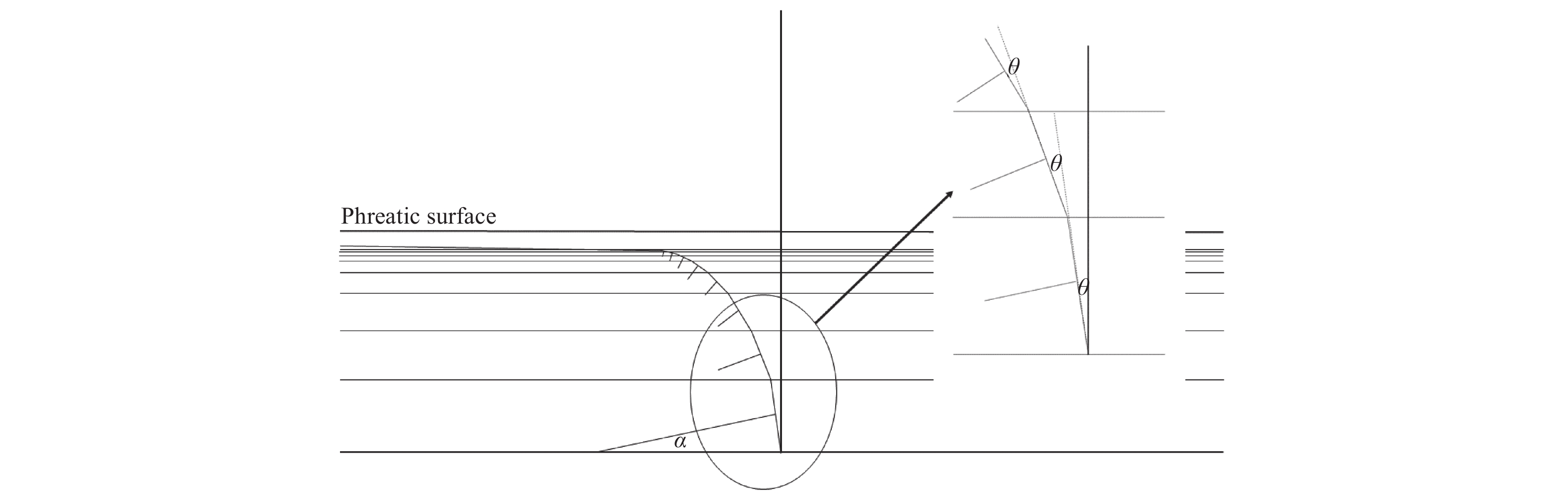
The high tensile strength, incompressibility, and ability of water to flow through the pore system govern soil deformation when tangential horizontal and compressive forces are applied to granular soils. We focused on the phreatic zone. Changes in the geometry of the soil (volumetric strain) due to bedrock displacement (Figure 1) cause water to flow through the connecting pores (incompressibility). For convenience, we treated this phenomenon as flow instead of soil strain.
Figure
1.
Schematic representation of the soil geometry changes during an oscillation (not to scale). ΔV represents the volume change, θ represents the geometry change (in the case of the intrinsic soil permeability not limiting the strain), ah is the horizontal acceleration of the bedrock, x is the bedrock displacement, and l is the phreatic surface height (reference: bedrock). The bottom images represent the bedrock acceleration, soil strain, and failure.
The geometry change is a function of the height of the phreatic surface (l), the bedrock displacement (x) and acceleration (ah), and the flux (q). The flux, as described by Darcy’s law, is a function of the intrinsic soil permeability (k), water viscosity (μ), the distance of any horizontal surface of interest (li) to the phreatic surface, and the pressure difference (∆p). Thus, the angle, θ, that defines the geometry change (for a shear deformation, (x/l ); Figure 1), keeping all but k constant, is ultimately a function of k (θ=f(k)). We assumed, for argument sake, that the domain of the function, the values of k (m2), is the interval [0, 1], then, in a given time for the motion (tm), for f(k) = arcsin(x/l), the limk→0f(k)=0 and limk→1f(k)=arcsin(x/l), i.e., no geometry change occurs when k approaches 0 m2, and a strain, independent of k, for the latter.
For each combination of the height of the phreatic surface (lps), the bedrock displacement (x) and horizontal acceleration (ah), the dry density of the soil (ρdd), and assuming that the contribution of the vadose zone is negligible, we can estimate the water pressure generated during the bedrock motion. The maximum pressure increase generated (∆pmax) can be estimated by Δpmax≈[ρdd×(lps/2)]×ah×sin45∘. The ∆pmax calculated this way may be insufficient for initiating any flow at higher depths below the phreatic surface. The flux (qmax) for this ∆pmax, defined for the horizontal soil surface where it first occurs (lflow), can now be calculated by Darcy’s law: qmax=−(k/μ)×{patm+[(l−lflow)×g×ρ]−Δpmax}/(l−lflow), where ρ is the water density, patm is the atmospheric pressure, and g is the gravitational acceleration. The estimated flux (qm) in time tm (tm=√x/a), and the potential volume change (∆V) are not equivalent. Thus, to ensure the continuity principle, at any given depth, if the estimated qm is higher than the potential volume change (∆V), we assume qm=∆V; otherwise, if qm is lower than ∆V, we assume ∆V=qm. The former (where qm>∆V) is only expected in soils of high intrinsic permeability. Both assumptions are speculative; however, the implications of these assumptions for the model are negligible.
The water pressure is normal to the soil strain plane (Figure 2), forming an angle α with the bedrock. As we move up the profile, the potential flux (qp)–in tm–increases, allowing for flux from the lower layers and that in that layer. Angle α increases. The ratio, qp / qm, for any height above the bedrock, provides a way to calculate α; for any surface of interest (li), αi = arctan(qpi / qmi).
Figure
2.
Schematic representation of the direction of the flow, perpendicular to the soil strain (not to scale). α is the angle between the direction of the water pressure (normal to the plane of soil strain) and the bedrock surface. The vertical line is a reference axis. During bedrock motion, for a given pressure, nearing the phreatic surface increases the potential flux beyond the actual flux, changing α.
At the depths that are likely to fail, q requires pressure differences higher than the effective load (σ' = (ρu × lu + ρdd × li) × g, where ρdd is the dry density of the soil) plus the atmospheric pressure. We set the pressure necessary for the flow to occur as ∆pr. If Δpr×sinα>(patm+σ′), the soil is lifted, and the contact points between the soil particles decrease, leading to plane failure. The failure plane has the highest potential volume change (∆V).
2.2
Reverse cyclic loading
If the pressure can sufficiently lift the soil, producing a ∆V value that is insufficient for a failure plane, further loadings may increase the total ∆V (ΔV=n∑i=1ΔVi, the sum of the ∆V of n loading cycles). If ∆V is sufficient for a failure plane, the pressure of the liquefied soil immediately below this surface equalizes the total load (the weight of the overburden per unit area plus the atmospheric pressure) as the diminishing load transfer through the soil particles occurs. The absolute pressure of liquefied soil (pls) becomes pls = patm + g × (ρs × ls + ρu × lu), where ls is the height from the failure plane to the phreatic surface. Most seismograms show one maximum oscillation, i.e., two maximum amplitudes in opposite directions (Rodkin and Orunbaev, 2022). Thus, the bulk of the volume change at the failure plane (∆V) is most likely reached during this oscillation; further oscillations, with smaller amplitude, most probably have a ∆V=0. The volume change is, at best, a few millimeters. Thus, in homogeneous soil, during an earthquake, the water flows, and the soil particles reconnect in a varying but short time.
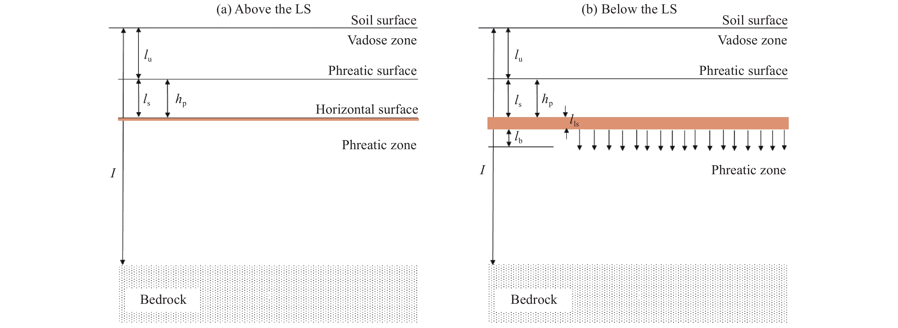
After the failure plane forms, two phenomena occur above and below the liquefied surface (Figure 3).
Figure
3.
Schematic representation of soil liquefaction triggering (not to scale). (a) Above the liquefied layer (at the interface with the non-liquefied soil), the water moves upward through the pores (the pressure difference is equivalent to the effective load of the overburden). (b) Below, the liquefaction front (the interface between the liquefied and non-liquefied soil, where the solid particles experience an effective load equal to zero (σ'=0)), the flux pushes and mixes the solid particles with the liquefied soil, and the interface recedes and eventually reaches the bedrock or another dense layer.
Below. The pressure (pb) of the water immediately below the liquefied layer at a distance (lb) (Figure 3b) can be calculated using pb = pls + (ρls×g × lls) + (ρ × g × lb), where ρls is the density of the liquefied soil and lls is the height of the liquefied layer. Because the load (of the overburden) is no longer transmitted through the solid particles immediately below the liquefied soil, the effective stress (σ'b) at a depth (lb) below the liquefied layer becomes σ′b=(g×lb×ρdd)−pb. Hence, limb→0σ′b=−pb, i.e., the effective stress, is σ’b = 0. In this context, the progressive loss of contact between the solid particles, beginning at the plane of failure and developing downward, is called the “liquefaction front”. As the loading cycles are repeated, the front may extend to the bedrock. The latter phenomenon depends on concurrent phenomena.
Above. If a failure occurs and pls<< ∆p, the hydraulic gradient between the failure plane and phreatic surface is equally lower (it becomes a function of the weight of the overburden); thus, for each loading cycle, the difference between the volume corresponding to the geometry change (qm, the flux arriving at the failure plane in time tm) and the flux upward corresponding to the new ∆p (pls) in time tm determines if the soil liquefies and for how long it persists in a homogeneous soil, i.e., how long it takes for the soil particles to reconnect at the failure plane. We can estimate the volume change at the failure plane (∆Vf), in time tm, for a given height of the failure plane below the phreatic surface lf, with the equation ΔVf=qm−[tm×(−k/μ)×((ρ×g×lf)+patm−pls)/lf]; if ∆Vf ≤0, the soil is not likely to liquefy; if ∆Vf >0, the number (and parameters) of the loading cycles determines the accumulated volume change and the time necessary for the particles to reconnect after end of the earthquake.
Two mechanisms are consistent with the model proposed to explain the persistence of liquefied soil. The existence of a lower permeability layer in the depth range in which the water pressure required for the flow is higher than the weight of the overburden negates the assumption of homogeneous soil. In the next section, the existence of these layers and their effects on different scenarios are discussed. In the worst-case scenarios studied, the time to revert liquefaction was only 1289 s, though it could be significantly higher, reaching hours. However, this mechanism does not explain the development of a liquefaction front because the volume change is too small, preventing the separation and loss of contact between soil particles. Thus, low-permeability layers at the depth range predicted to produce failure planes can explain the persistence of soil liquefaction after an earthquake, but not the significant liquefaction of the whole profile or layer width.
A mechanism for homogeneous soils requires water inflow from the bedrock springs. The existence of active bedrock springs (artesian water) before the earthquake means that the artesian water pressure is sufficient for water flow. If we ignore the pore water pressure induced by the bedrock motion, when a failure plane occurs, the artesian pressure necessary for the spring flow must be higher than the combined pressure of the water column (phreatic width) plus the effective stress at the failure plane. This continuous water flow from the bedrock springs contributes to the volume change and development of the liquefaction front from top to bottom. Thus, two scenarios were possible. First, the pressure was insufficient, and the flow stopped. In this situation, the downward liquefaction front did not develop because the volume changes following the peak oscillations were small. In the second, the artesian pressure is sufficient for water to keep flowing, and a liquefaction front extends from the failure plane towards the bedrock, accompanied by the growth of the flow rate as the non-liquefied width diminishes; eventually, the effective stress of the non-liquefied soil is lower than the artesian pressure, and this layer is promptly mixed in the above-liquefied layer (and the spring flow rate increases exponentially). The flow rate (and water volume in the cavities above the springs) of these springs defines how long the liquefied soil persists and the volume affected. In the bedrock springs and outflow pathways, the environmental effects of soil liquefaction can be explained by this mechanism; for example, liquefied soil may enter the hydraulic pathways (springs and outflows) and become clogged, causing changes in the phreatic surface levels during earthquakes that may persist for long periods after the event.
3.
Simulation (calculation)
In this section, we consider all the assumptions made previously. The soil and profile properties and horizontal accelerations are listed in Table 1.
Table
1.
Soil and profile properties, maximum horizontal acceleration, dynamic viscosity (Kestin et al., 1978).
Parameter
Intrinsic permeability
k= 10−10 m2
k= 10−11 m2
k= 10−12 m2
Soil porosity (Vp/V)
0.45
0.45
0.48
Water content (drained soil) (Vw/V)
0.16
0.2
0.22
Density soil particles (kg·m−3)
2700
2700
2700
Density unsaturated soil (kg·m−3)
1645
1685
1624
Density saturated soil (kg·m−3)
1935
1935
1884
Dynamic viscosity (5 °C) (Pa·s)
1.52 x 10⁻³
Width of the vadose zone (VZ) (m)
2.5, 5 and 10
Width of the phreatic zone (PZ) (m)
30, 50 and 100
Bedrock displacement (x) (m)
1, 2.5 and 5
Horizontal acceleration of the bedrock (ah) (m·s−2)
Using Darcy’s law, the pressure required for a given flux to occur given a set of conditions can be calculated easily. Considering the profile features (width of the phreatic and vadose zones), bedrock displacement, and horizontal accelerations, soils with an intrinsic permeability equal to or higher than 10−9 m2 did not yield horizontal failure planes because the pressure required for the flow was lower than the effective stress. The depth ranges in which failure planes may occur in various scenarios are listed in Table 2. It is apparent that the profile features (phreatic zone and vadose width) and bedrock motion features (acceleration) determine these depth ranges independently of the intrinsic permeability of the soils; that is, the magnitude of the differences in the soil parameters used to calculate the water pressure and effective load is small. As expected, a higher bedrock acceleration diminished the height above the bedrock at which a failure plane occurs (higher water pressure). For the highest bedrock accelerations (24.4 m·s−2), failure planes are predicted for profiles with phreatic zone widths as low as 30 m and vadose widths of 2.5 m. An Excel sheet is provided in the Supplementary Materials, which allows the reader to replicate or create these simulations.
Table
2.
Depth range for which the pressure necessary for the flow is higher than the weight of the overburden Δpr×sinα>(patm+σ′).
k= 10−10 m2
k= 10−11 m2
k= 10−12 m2
Horizontal acceleration
Horizontal acceleration
Horizontal acceleration
12.2 m·s−2
24.4 m·s−2
12.2 m·s−2
24.4 m·s−2
12.2 m·s−2
24.4 m·s−2
PZ
BRD
VZ
lf Min
lf Max
lf Min
lf Max
lf Min
lf Max
lf Min
lf Max
lf Min
lf Max
lf Min
lf Max
100
1
2.5
90
96
68
98
89
99
68
99
90
99
69
99
5
70
98
91
98
70
99
92
99
71
99
10
74
97
95
97
74
99
96
99
75
99
2.5
2.5
89
98
68
99
89
99
68
99
90
99
69
99
5
91
98
70
99
91
99
70
99
92
99
71
99
10
74
98
95
99
74
99
96
99
75
99
5
2.5
89
99
68
99
89
99
68
99
90
99
69
99
5
91
99
70
99
91
99
70
99
92
99
71
99
10
95
98
74
99
95
99
74
99
96
99
75
99
50
1
2.5
39
48
39
49
40
49
5
41
48
41
49
42
49
10
45
46
45
49
46
49
2.5
2.5
39
49
39
49
40
49
5
41
49
41
49
42
49
10
45
48
45
49
46
49
5
2.5
39
49
39
49
40
49
5
41
49
41
49
42
49
10
45
49
45
49
46
49
30
1
2.5
28
28
29
28
29
5
-
-
-
-
-
-
10
-
-
-
-
-
-
2.5
2.5
28
29
28
29
28
29
5
-
-
-
-
-
-
10
-
-
-
-
-
-
5
2.5
28
29
28
29
28
29
5
-
-
-
-
-
-
10
-
-
-
-
-
-
Note: lf is the height above the bedrock of the plane predicted to fail (m); PZ is the phreatic zone width (m); BRD is bedrock displacement (m); and VZ is the width of the vadose zone (m). Read from left to right, characters in bold represent 90 to 96 m above bedrock, for phreatic and vadose widths of 100 m and 2.5 m, respectively, and for an intrinsic permeability of 10−10 m2 and a bedrock acceleration and displacement of 12.2 m·s−2 and 1 m, respectively. bedrock is the reference surface; 0 m.
The volume changes (∆Vf), in case of failure plane and for a half cycle (motion in one direction), are presented in Table 3. For all soils, ∆Vf increases for heights nearer the phreatic surface, but it may or may not be the nearest. The ranges of heights above the bedrock for the failure planes to occur (Table 2), and the volume changes at those heights in the case of failure were calculated based on the assumption of cohesionless soils. Very fine soils (for example clay) show cohesion and a shrink-swell behavior; the volume changes calculated for these soils (with k≈10−13 m2) are, in the scenarios with the highest ∆Vf, approximately 30 μm and are unlikely to reduce the soil strength significantly (i.e., to reduce the number of contact points between the particles).
Table
3.
Volume change ranges (∆Vf, m=m3/m2).
k= 10−10 m2
k= 10−11 m2
k= 10−12 m2
Horizontal acceleration
Horizontal acceleration
Horizontal acceleration
12.2 m·s−2
24.4 m·s−2
12.2 m·s−2
24.4 m·s−2
12.2 m·s−2
24.4 m·s−2
PZ
BRD
VZ
∆Vf Min
∆Vf Max
∆Vf Min
∆Vf Max
∆Vf Min
∆Vf Max
∆Vf Min
∆Vf Max
∆Vf Min
∆Vf Max
∆Vf Min
∆Vf Max
100
1
2.5
0.00058
0.00076
0.00028
0.00125
0.00006
0.00030
0.00003
0.00044
0.00001
0.00008
0.00000
0.00012
5
0.00029
0.00111
0.00007
0.00025
0.00003
0.00039
0.00001
0.00008
0.00000
0.00011
10
0.00033
0.00092
0.00011
0.00017
0.00003
0.00033
0.00001
0.00006
0.00000
0.00010
2.5
2.5
0.00092
0.00282
0.00044
0.00422
0.00009
0.00095
0.00004
0.00134
0.00001
0.00013
0.00000
0.00022
5
0.00108
0.00231
0.00046
0.00379
0.00011
0.00083
0.00005
0.00125
0.00001
0.00012
0.00000
0.00021
10
0.00052
0.00320
0.00018
0.00058
0.00005
0.00107
0.00002
0.00010
0.00001
0.00020
5
2.5
0.00130
0.00712
0.00063
0.01039
0.00013
0.00204
0.00006
0.00284
0.00001
0.00019
0.00001
0.00031
5
0.00153
0.00542
0.00066
0.00919
0.00015
0.00186
0.00007
0.00272
0.00002
0.00017
0.00001
0.00030
10
0.00257
0.00417
0.00073
0.00794
0.00025
0.00151
0.00007
0.00247
0.00003
0.00014
0.00001
0.00028
50
1
2.5
0.00041
0.00153
0.00004
0.00048
0.00000
0.00006
5
0.00048
0.00127
0.00005
0.00043
0.00001
0.00005
10
0.00077
0.00087
0.00008
0.00032
0.00001
0.00004
2.5
2.5
0.00065
0.00513
0.00006
0.00102
0.00001
0.00009
5
0.00077
0.00428
0.00008
0.00093
0.00001
0.00009
10
0.00128
0.00303
0.00013
0.00076
0.00002
0.00007
5
2.5
0.00092
0.01141
0.00009
0.00144
0.00001
0.00013
5
0.00108
0.01020
0.00011
0.00132
0.00001
0.00012
10
0.00182
0.00780
0.00018
0.00107
0.00002
0.00010
30
1
2.5
0.00135
0.00014
0.00030
0.00001
0.00003
5
-
-
-
-
-
-
10
-
-
-
-
-
-
2.5
2.5
0.00225
0.00480
0.00022
0.00048
0.00002
0.00004
5
-
-
-
-
-
-
10
-
-
-
-
-
-
5
2.5
0.00318
0.00679
0.00032
0.00068
0.00003
0.00006
5
-
-
-
-
-
-
10
Note: ∆V is volume change (m); PZ is phreatic zone width (m); BRD is bedrock displacement (m); VZ is vadose zone width (m). Read from left to right, characters in bold represent volume changes of 5.8 × 10⁻⁴ to 7.6 × 10⁻⁴ m, for phreatic and vadose widths of 100 m and 2.5 m, respectively, and for intrinsic permeability of 10−10 m2 and a bedrock acceleration and displacement of 12.2 m·s−2 and 1 m, respectively.
The plane that is likely to fail is the one for which the volume change is the highest after half a cycle (motion in one direction). These pairs are listed in Table 4.
Table
4.
Height above the bedrock of the plane that is predicted to fail (lf) and the volume change (∆Vf).
k= 10−10 m2
k= 10−11 m2
k= 10−12 m2
Horizontal acceleration
Horizontal acceleration
Horizontal acceleration
12.2 m·s−2
24.4 m·s−2
12.2 m·s−2
24.4 m·s−2
12.2 m·s−2
24.4 m·s−2
PZ
BRD
VZ
lf
∆Vf
lf
∆Vf
lf
∆Vf
lf
∆Vf
lf
∆Vf
lf
∆Vf
100
1
2.5
96
0.00076
97
0.00125
99
0.00030
99
0.00044
99
0.00008
99
0.00012
5
95
0.00111
98
0.00025
98
0.00039
99
0.00008
99
0.00011
10
93
0.00092
97
0.00017
98
0.00033
99
0.00006
99
0.00010
2.5
2.5
98
0.00282
98
0.00422
99
0.00095
99
0.00134
99
0.00013
99
0.00022
5
97
0.00231
98
0.00379
99
0.00083
99
0.00125
99
0.00012
99
0.00021
10
97
0.00320
99
0.00058
99
0.00107
99
0.00010
99
0.00020
5
2.5
99
0.00712
99
0.01039
99
0.00204
99
0.00284
99
0.00019
99
0.00031
5
99
0.00542
99
0.00919
99
0.00186
99
0.00272
99
0.00017
99
0.00030
10
98
0.00417
98
0.00794
99
0.00151
99
0.00247
99
0.00014
99
0.00028
50
1
2.5
48
0.00153
49
0.00048
49
0.00006
5
48
0.00127
49
0.00043
49
0.00005
10
46
0.00087
49
0.00032
49
0.00004
2.5
2.5
49
0.00513
49
0.00102
49
0.00009
5
49
0.00428
49
0.00093
49
0.00009
10
48
0.00303
49
0.00076
49
0.00007
5
2.5
49
0.01141
49
0.00144
49
0.00013
5
49
0.01020
49
0.00132
49
0.00012
10
49
0.00780
49
0.00107
49
0.00010
30
1
2.5
28
0.00135
29
0.00030
29
0.00003
5
-
-
-
-
-
-
10
-
-
-
-
-
-
2.5
2.5
29
0.00480
29
0.00048
29
0.00004
5
-
-
-
-
-
-
10
-
-
-
-
-
-
5
2.5
29
0.00679
29
0.00068
29
0.00006
5
-
-
-
-
-
-
10
Note: ∆V is volume change (m); lf is height above the bedrock of the plane predicted to fail (m); PZ is phreatic zone width (m); BRD is bedrock. Read from left to right, characters in bold represent 96 m above the bedrock (4 m below the phreatic surface) and a volume change of 7.6 × 10⁻⁴ m, for phreatic and vadose widths of 100 m and 2.5 m, respectively, and for intrinsic permeability of 10−10 m2 and a bedrock acceleration and displacement of 12.2 m·s−2 and 1 m, respectively. displacement (m); VZ is vadose zone width (m). The bedrock is the reference surface (0 m).
The persistence of the volume change, assuming that further cycles would not contribute to the volume, was a few seconds, with a maximum of 11 seconds (Table 5).
Table
5.
Persistence (s) for the volume change ranges (∆Vf, m=m3/m2).
k= 10−10 m2
k= 10−11 m2
k= 10−12 m2
Horizontal acceleration
Horizontal acceleration
Horizontal acceleration
12.2 m·s−2
24.4 m·s−2
12.2 m·s−2
24.4 m·s−2
12.2 m·s−2
24.4 m·s−2
PZ
BRD
VZ
tmin
tmax
tmin
tmax
tmin
tmax
tmin
tmax
tmin
tmax
tmin
tmax
100
1
2.5
1.07
1.30
1.25
1.97
1.27
2.36
1.65
3.51
3.23
3.23
4.26
4.62
5
1.01
1.38
1.10
1.40
1.48
2.13
1.69
1.69
2.23
2.52
10
0.71
0.88
0.72
0.77
0.78
1.20
0.87
0.87
1.14
1.32
2.5
2.5
2.17
3.11
2.89
4.62
3.58
4.63
4.73
6.70
5.11
5.11
8.04
8.04
5
1.56
1.93
1.60
2.97
1.89
2.55
2.49
3.80
2.68
2.68
4.21
4.21
10
1.15
1.75
0.97
1.35
1.28
2.05
1.37
1.37
2.16
2.16
5
2.5
3.04
5.44
3.96
8.18
7.35
7.35
9.82
10.33
7.23
7.23
11.37
11.37
5
2.62
3.21
2.09
4.90
3.88
3.88
5.18
5.70
3.79
3.79
5.96
5.96
10
1.38
1.77
1.87
2.76
1.99
1.99
2.66
3.00
1.94
1.94
3.05
3.05
50
1
2.5
1.14
1.50
1.80
2.07
2.29
2.29
5
0.63
0.92
0.95
1.14
1.20
1.20
10
0.49
0.52
0.49
0.60
0.61
0.61
2.5
2.5
2.05
2.99
3.68
3.68
3.61
3.61
5
1.08
1.72
1.94
1.94
1.89
1.89
10
0.86
0.93
1.00
1.00
0.97
0.97
5
2.5
4.30
4.72
5.20
5.20
5.11
5.11
5
2.27
2.61
2.74
2.74
2.68
2.68
10
1.17
1.38
1.41
1.41
1.37
1.37
30
1
2.5
1.03
1.03
1.20
1.20
1.17
1.17
5
-
-
-
-
-
-
10
-
-
-
-
-
-
2.5
2.5
1.94
1.94
1.90
1.90
1.84
1.84
5
-
-
-
-
-
-
10
-
-
-
-
-
-
5
2.5
2.74
2.74
2.68
2.68
2.61
2.61
5
-
-
-
-
-
-
10
-
-
-
-
-
-
Note: PZ is phreatic zone width (m); BRD is bedrock displacement (m); VZ is vadose zone width (m). Read from left to right, characters in bold represent minimum and maximum persistence time, for phreatic and vadose widths of 100 m and 2.5 m, respectively, and for intrinsic permeability of 10−10 m2 and a bedrock acceleration and displacement of 12.2 m·s−2 and 1 m, respectively.
The existence of a soil layer of low permeability in the range of heights predicted to fail affects the persistence of the volume change. Table 6 presents the time necessary for the flow of the volume change in the plane with the highest probability of failure (lf) (Table 4) in the presence of a layer with an intrinsic permeability of k= 10−13 m2 and width of 0.3 m. The persistence was longer in soil with higher permeability, approximately 1289 s, and, keeping all other variables constant, decreased for successively lower permeabilities. This pattern is explained by the significantly higher magnitude of volume change for soils with higher permeability.
Table
6.
Time to revert liquefaction (∆V/q) for permeabilities (k) of 1 × 10⁻¹⁰ to 1 × 10⁻¹² m2, in the presence of a layer of lower permeability with a k= 10−13 m2 and a width of 0.3 m on top of the plane that is likely to fail (lf) (Table 4).
k= 10−10 m2
k= 10−11 m2
k= 10−12 m2
Horizontal acceleration
Horizontal acceleration
Horizontal acceleration
12.2 m·s−2
24.4 m·s−2
12.2 m·s−2
24.4 m·s−2
12.2 m·s−2
24.4 m·s−2
PZ
BRD
VZ
t
∆Vf
t
∆Vf
t
∆Vf
t
∆Vf
t
∆Vf
t
∆Vf
100
1
2.5
80
0.00076
125
0.00125
38
0.00030
49
0.00044
10
0.00008
13
0.00012
5
61
0.00111
17
0.00025
22
0.00039
5
0.00008
7
0.00011
10
30
0.00092
7
0.00017
12
0.00033
3
0.00006
3
0.00010
2.5
2.5
326
0.00282
434
0.00422
107
0.00095
142
0.00134
15
0.00013
24
0.00022
5
156
0.00231
240
0.00379
57
0.00083
75
0.00125
8
0.00012
13
0.00021
10
115
0.00320
29
0.00058
38
0.00107
4
0.00010
6
0.00020
5
2.5
912
0.00712
1187
0.01039
221
0.00204
295
0.00284
22
0.00019
24
0.00031
5
393
0.00542
626
0.00919
116
0.00186
155
0.00272
11
0.00017
18
0.00030
10
207
0.00417
280
0.00794
60
0.00151
80
0.00247
6
0.00014
9
0.00028
50
1
2.5
171
0.00153
54
0.00048
7
0.00006
5
94
0.00127
28
0.00043
4
0.00005
10
37
0.00087
15
0.00032
2
0.00004
2.5
2.5
615
0.00513
110
0.00102
11
0.00009
5
324
0.00428
58
0.00093
6
0.00009
10
129
0.00303
30
0.00076
3
0.00007
5
2.5
1289
0.01141
156
0.00144
15
0.00013
5
680
0.01020
82
0.00132
8
0.00012
10
350
0.00780
42
0.00107
4
0.00010
30
1
2.5
154
0.00135
36
0.00030
3
0.00003
5
-
-
-
-
-
-
10
-
-
-
-
-
-
2.5
2.5
582
0.00480
57
0.00048
6
0.00004
5
-
-
-
-
-
-
10
-
-
-
-
-
-
5
2.5
823
0.00679
81
0.00068
8
0.00006
5
-
-
-
-
-
-
10
-
-
-
Note: ∆V is volume change (m); PZ is phreatic zone width (m); BRD is bedrock displacement (m); VZ is vadose zone width (m). Read from left to right, characters in bold represent the 1289 s to revert liquefaction, for a layer of lower permeability on top of the plane likely to fail (49 m, in Table 4), for phreatic and vadose widths of 50 m and 2.5 m, respectively, and for intrinsic permeability of 10−10 m2 and a bedrock acceleration and displacement of 24.4 m·s−2 and 5 m, respectively.
The results in Table 6 are not consistent with reports of the persistence of liquefaction hours after an earthquake, particularly if the soil permeability is relatively low (or inferred to be low), such as silts in the Christchurch earthquake of 2010–2011 (Cox et al., 2021). In the scenario with the highest persistence (k=10−10 m2, PZ=50 m, VZ=2.5 m, BRD= 5 m, and ah=24.4 m·s−2), a 1-m soil layer with low permeability (from the predicted failed plane to the phreatic surface), would increase the persistence to 4297 s; for the same setting, in soils with lower permeability, k=10−11 and 10−12 m2, it would be 520 and 51 s, respectively. Increasing the layer width to explain the persistence is possible but limited because it must be located above the lower bound of the range of depths for which the planes may fail. Moreover, while increasing the width, the potential volume change decreases. However, using the example with the highest ∆Vf, a volume change of 0.011 m allows for the liquefaction of a limited width below the failed plane. Thus, even in the presence of almost impervious layers, a mechanism is still required to explain the development of liquefaction.
In homogeneous soils, water inflow from the bedrock springs is necessary to explain the persistence of liquefaction. Table 7 presents the results (an oversimplification) of the flux in the interface between the liquefied and non-liquefied soils, the maximum manometric pressure of the bedrock springs, the flow rate of the bedrock springs, and the interface area between the bedrock spring and the soil (for example, the surface area of a cavity above the spring) necessary to maintain liquefaction in a projected area (surficial) of 1000 m2, for the worst scenario discussed above (k=10−10 m2, PZ=50 m, VZ=2.5 m, BRD= 5 m, and ah=24.4 m·s−2) and for soils of lower permeability (keeping the other parameters constant). In homogenous soils, despite the differences in the flux at the interface between non-liquefied and liquefied soils and the flow rate (Q) of the bedrock spring, the necessary interface area at the bedrock springs is similar for all soils and approximately 3.4 times the affected surface (1000 m2); however, a layer of low permeability (k=10−13 m2 and 0.3 m width) on top of the failure plane has a profound effect on the required interface area at the bedrock springs: 11, 115, and 349 m2, for k=10−10, 10−11, and 10−12 m2, respectively. In these scenarios, the bedrock-spring interface areas and pressure heads govern the persistence of volume changes and the development of a liquefaction front. Once the soil is liquefied to a depth at which the effective load above the bedrock is lower than the pressure head of the spring, the sudden Q increase stirs up the liquefied soil, explaining “instant” liquefaction events. The liquefied state persists until the artesian pressure drops below the necessary pressure.
Table
7.
Bedrock springs flow rate necessary to allow soil liquefaction persistence and development, in a projected area of 1000 m2 affected by liquefaction (surficial) with PZ=50 m, VZ=2.5 m, BRD= 5 m and ah=24.4 m·s−2.
k= 10−10 m2
k= 10−11 m2
k= 10−12 m2
Homogenous
fsq (m·s−1)
2.97 × 10⁻³
3.03 × 10⁻⁴
2.88 × 10⁻⁵
p (Pa)
1.3 × 10⁶
1.3 × 10⁶
1.2 × 10⁶
Q (m3·s−1)
2.967
0.303
0.029
Area brs (m2)
3379
3447
3491
Layered
fsq (m·s−1)
9.89 × 10⁻⁶
1.01 × 10⁻⁵
2.88 × 10⁻⁶
Q (m3·s−1)
0.010
0.010
0.003
Area brs (m2)
11
115
349
Note: fsq (m·s−1) is flux through the interface between liquefied and non-liquefied soil; p (Pa) is maximum manometric artesian water pressure for flux (at the bedrock springs); Q (m3·s−1) is flow rate from the bedrock springs; Area brs (m2) is area of the interface above the bedrock springs transmitting the flux.
In the volume of influence of the bedrock spring, the relationship between the water pressure (artesian), the width of the phreatic zone, and the water pressure resulting from the bedrock acceleration and displacement are complex and outside the scope of this study.
4.
Discussion
The current empirical framework for assessing the potential resistance of soil to liquefaction (Youd et al., 2001) is based on assumptions for which there is insufficient evidence. One such assumption is that the soil liquefaction triggering and development and the surficial effects observed share the same mechanism (Youd et al., 2001). Previous studies have questioned the current framework for explaining soil liquefaction based on observations that do not conform to the mechanisms implicit in the framework, such as locations too distant from the hypocenter of an earthquake (low seismic energy density; Wang CY et al. (2006), Wang CY (2007). The proposed mechanisms for triggering the development of a liquefaction front and persistence provide a theoretical approach to studying these observations, including surficial effects.
The empirical equation for the cyclic stress ratio for an earthquake with a moment magnitude (MW) of 7.5 is the standard procedure for studying soil resistance to liquefaction (Youd et al., 2001). For a meaningful comparison with the proposed model, a relationship must be first established between the observed maximum horizontal acceleration at the ground surface and that of the bedrock. Other critical factors necessary for the analysis are the intrinsic permeability of the soil, width of the profile (bedrock to ground surface), depth of the phreatic surface, existence and depth distribution of layers of different permeabilities, and existence of bedrock water springs (and their features) at the locations where liquefaction occurred. Unfortunately, the available databases lack data but allow us to discuss the validity of certain aspects of the model. For example, in the database of the 2008 Wenchuan earthquake provided by Zhou YG et al. (2020), the gravel content of these soils has arithmetic means of 30% and 37% in liquefied and non-liquefied soils, respectively, prompting a discussion on the liquefaction resistance of gravelly soils assuming that highly permeable soils are resistant to liquefaction. However, by assuming a water temperature, for example, 5 °C, the intrinsic permeability of the soils can be calculated from the permeabilities reported in the database; for this water temperature, their arithmetic means are 5.5 × 10⁻¹¹ and 5.9 × 10⁻¹¹ m2, in liquefied and non-liquefied locations, respectively, i.e., low intrinsic permeabilities when compared to uniformly-graded gravels. Other parameters of the Wenchuan earthquake database consistent with the present model are the phreatic surface depth, 2.9 and 4.2 m, and peak ground acceleration at the ground surface (PGA), 0.57 g and 0.33 g, in liquefied and non-liquefied soils, respectively (both statistically significantly different for α<0.05). In another database by Cetin et al. (2018), covering 19 earthquakes worldwide, the arithmetic means and standard errors of various parameters were similar between the two groups (113 liquefaction and 97 non-liquefaction events). The exceptions are the mean value of the standard penetration test (SPT) blow count–that of the non-liquefied soil is approximately twice that observed in liquefied soils–and the shear wave velocity for the upper 12 m. Both are consistent with the present model. Unfortunately, we cannot infer the intrinsic permeability of the soils or the width of the soil profile from the data without unacceptable speculation; thus, we offer no counterargument. However, one can speculate that the critical depths identified with the SPT (more susceptible to liquefaction) correspond to the range of depths for which the failure plane is predicted by the model, i.e., the depths in the soil profile that have been ruptured by previous earthquakes (the soil liquefies, but a liquefaction front does not necessarily develop). A relationship between inherent soil properties already in the databases, the intrinsic permeability and profile width (from the ground surface to the bedrock) would allow the data to be reinterpreted using the proposed model. Such a relationship may be difficult, expensive, and time-consuming to establish. However, a systematic measurement (or compilation from technical reports) of the intrinsic permeability of the layers that constitute the profiles and the depth from the ground surface to the bedrock of these historical events (integrating such databases) should be considered in the future.
At the moment of failure (i.e., soil liquefaction at that plane), one can hypothesize that uniformly-graded soils have a significantly sharper water pressure change (the load transfer to the bedrock changes from interparticle to water) than well-graded soils because of the fast loss of contact between the particles when compared to soils with particles of different sizes moving and occupying the spaces between larger particles transmitting, at least partially, the load. Experimental observations supporting this hypothesis exist in the literature, albeit with different interpretations of the results. The volume change necessary to unlock the soil particles at the failure plane requires the pore water pressure to be higher than the effective stress. However, the pore water pressure and persistence are inconsistent in soils with high intrinsic permeability (Sturm and DeJong, 2020). Soils with extremely low intrinsic permeabilities (e.g., clays) allow for high water pressure, which is consistent with the proposed model; however, because of the small volume change, even if a failure plane occurs, its persistence would be small, and the development of a liquefaction front would require particular circumstances.
Based on the mechanisms presented, once the liquefied layer (plane) is established and the permeability and volume change allow for the persistence of this liquefied state, horizontal acceleration (further oscillations) cause the contact between the particles to be lost from the top to bottom if an inflow of water (bedrock springs) is provided. The concept of a liquefaction front has been observed in laboratory experiments (González et al., 2005). When the data of the experiment, a centrifuge model (parameters of Model 1 in González et al. (2005)), are tested with the proposed model, with only a few assumptions to remediate the lack of data, such as a water temperature of 5 °C, to calculate k (1.55 × 10⁻¹¹ m2) from the permeability, an average particle density of 2700 kg·m−3, a bedrock displacement of 0.01 m, and a gravitational acceleration of 120 g, the initial failure plane depth is predicted accurately, 0.004 m below the phreatic surface and after half a cycle (oscillation in one direction). This corresponds to a volume change of 0.0033 m. The authors observed a failure plane at 0.013 m after two cycles of shaking, the depth corresponding to the first pressure sensor. However, the liquefaction front observed in the experiment cannot be attributed to the proposed mechanism, as there was no water inflow, and the separation of the two soil phases was likely caused by the extreme centrifuge acceleration of the sample (120 g). To replicate the results, use the model in the Supplemental Materials.
According to the model, in very deep aquifers, a liquefaction front extending from the plane of failure (a necessary condition) to the bedrock requires significant pressure heads at the bedrock springs. Wang CY (2007) cited a report by the Water Conservancy Agency of China regarding changes in the water levels of three wells (at depths of 126, 198, and 258 m) before the 1999 Chi-Chi (Jiji) earthquake, which were similar in the aftermath. An interpretation of the insufficient data, consistent with the proposed model, suggests clogging of the outflow pathways by liquefied soil and a new hydrostatic equilibrium. The magnitude of the Chi-Chi (Jiji) earthquake was 7.6 (MW), but this relays little information regarding the bedrock displacement and acceleration. Li WH et al. (2019) reported displacements of 10 m and velocities of 3–5 m·s−1 for a fault, and an inland earthquake with displacements of several meters and velocities of approximately 1 m·s−1. The epicenter was surrounded by high peaks (many above 3000 m), suggesting the presence of pressure heads of convenient magnitude. If these values are tested with the proposed model– for a profile width of 258 m, a bedrock acceleration and displacement of 24.4 m·s−2 and 10 m, and k=10−10 m2– the lower bound of the range of depths for which failure planes may occur, is approximately 162 m, meaning that soil liquefaction may occur without observable surficial effects; the soil damping would reduce the surficial acceleration and amplitude of the oscillations.
A three-dimensional analysis of the proposed mechanisms at the microscale (a representative volume element) requires connecting the displacement field of the solid particles, pore geometry change, and associated flux (pore volume reduction). If successful, it would allow a better understanding of the mechanism of plane failure and the interplay between the pore water pressure generated because of the soil horizontal acceleration, the flux generated, and the flux from the artesian springs. Current constitutive equations for sand to determine its response to loads regarding the evolution of porosity and pore water pressure are built upon flow plasticity theories (Papadimitriou and Bouckovalas, 2002). These equations require several input parameters that can only be determined experimentally and were guided by assumptions and boundary conditions that do not entirely coincide with those of the proposed mechanisms. The intrinsic permeability of soil is central to creating adequate constitutive equations and defining boundary conditions to describe the soil response to loads. In this context, the state parameter (ψ) of Been and Jefferies (1985) and other variables and ratios should be revisited from this new perspective. In saturated soils, the soil strength and strain are controlled by the flux; the pore volume reduction affects the intrinsic permeability of the soil, and thus the flux (however, this effect is deemed small at a macro scale). In the proposed framework, water tensile strength is a key concept for understanding soil behavior when subjected to horizontal acceleration.
The bedrock horizontal acceleration (peak) and displacement can be estimated theoretically or empirically based on surface measurements of horizontal acceleration and oscillation amplitude. The proposed triggering mechanism reduces the soil shear strength (for granular soil) or the perceived angle of internal friction (soil lifted by water pressure). The failure of the horizontal plane during peak oscillation likely increases soil damping beyond the values predicted by the current models.
5.
Conclusions
The mechanisms proposed for the triggering, persistence, and development of soil liquefaction exhibited physically consistent parameter values. The predictions made for liquefaction triggering, given a set of profile and bedrock motion features (soil depth, phreatic surface depth, maximum bedrock horizontal acceleration, and displacement) and soil properties (intrinsic permeability), allow for the identification of depths below the phreatic surface of the planes that are most likely to fail and explain the nature of the resistance of soils to liquefaction (insufficient pore water pressure for high intrinsic permeability soils and insufficient volume change for low intrinsic permeabilities). The persistence of the liquefied state in the failure plane was low in the homogeneous soils. When it extends for more than a few seconds, it requires low (lower) permeability layers in the range predicted to fail, and the effect of such layers is greater in more permeable soils (in absolute terms). The development of liquefaction, the concept of a liquefaction front, requires water inflow from bedrock springs; it has a double effect, providing the volume change necessary for liquefaction and increasing its persistence. Soils with higher permeability require smaller bedrock spring interface areas with the soil.
The databases on the historical records of earthquake-induced soil liquefaction lack fundamental parameters to prove or refine the proposed mechanisms, i.e., the soil intrinsic permeability and depth (to the bedrock). Soil grain size distribution is a poor variable for inferring the resistance of a given soil to liquefaction, and soils with relatively high gravel content may have low intrinsic permeability.
The problem of bedrock horizontal acceleration and displacement estimation, and their relationship with surface measurements of the acceleration and amplitude of the oscillation, given the mechanism proposed for the failure plane, should be addressed.
The model proposed is based on the flux characteristics and the effective stress experienced by the soil particles at the plane of failure, reducing the soil shear strength. However, low-permeability layers and bedrock springs are required for soil liquefaction development and persistence through the soil profile. If this model (hypothesis) represents the phenomenon, the soil liquefaction risk assessment can be achieved by surveying the parameters needed for each mechanism.
Acknowledgement
I want to express my utmost gratitude to all who supported my work.
Conflict of interest
The author affirms that there are no financial and personal relationships with any individual or organization that could have potentially influenced the work presented in this paper.
Cetin KO, Seed RB, Kayen RE, Moss RES, Bilge HT, Ilgac M and Chowdhury K (2018). Dataset on SPT-based seismic soil liquefaction. Data Brief 20: 544 – 548 . https://doi.org/10.1016/j.dib.2018.08.043.
Cox SC, Van Ballegooy S, Rutter HK, Harte DS, Holden C, Gulley AK, Lacrosse V and Manga M (2021). Can artesian groundwater and earthquake-induced aquifer leakage exacerbate the manifestation of liquefaction? Eng Geol 281: 105982 . https://doi.org/10.1016/j.enggeo.2020.105982.
González L, Abdoun T, Zeghal M, Kallou V and Sharp MK (2005). Physical modeling and visualization of soil liquefaction under high confining stress. Earthq Engin Engin Vib 4(1): 47 – 57 . https://doi.org/10.1007/s11803-005-0023-x.
Isobe K, Ohtsuka S and Nunokawa H (2014). Field investigation and model tests on differential settlement of houses due to liquefaction in the Niigata-ken Chuetsu-Oki earthquake of 2007. Soils Found 54(4): 675 – 686 . https://doi.org/10.1016/j.sandf.2014.06.022.
Kestin J, Sokolov M and Wakeham WA (1978). Viscosity of liquid water in the range −8 °C to 150 °C. J Phys Chem Ref Data 7(3): 941 – 948 . https://doi.org/10.1063/1.555581.
LeBoeuf D, Duguay-Blanchette J, Lemelin JC, Péloquin E and Burckhardt G (2016). Cyclic softening and failure in sensitive clays and silts. In: Proceedings of the 1st International Conference on Natural Hazards and Infrastructure. Chania, Greece, https://www.researchgate.net/profile/Eric-Peloquin/publication/304497959_CYCLIC_SOFTENING_AND_FAILURE_IN_SENSITIVE_CLAYS_AND_SILTS/links/5773e0ec08ae4645d60a07a0/CYCLIC-SOFTENING-AND-FAILURE-IN-SENSITIVE-CLAYS-AND-SILTS.pdf.
Li WH, Lee CH, Ma MH, Huang PJ and Wu SY (2019). Fault Dynamics of the 1999 Chi-Chi earthquake: clues from nanometric geochemical analysis of fault gouges. Sci Rep 9: 5683 . https://doi.org/10.1038/s41598-019-42028-w.
Liu AW, Chen K and Wu J (2010). State of art of seismic design and seismic hazard analysis for oil and gas pipeline system. Earthq Sci 23(3): 259 – 263 . https://doi.org/10.1007/s11589-010-0721-y.
Papadimitriou AG and Bouckovalas GD (2002). Plasticity model for sand under small and large cyclic strains: A multiaxial formulation. Soil Dyn Earthq Eng 22(3): 191 – 204 . https://doi.org/10.1016/S0267-7261(02)00009-X.
Rodkin MV and Orunbaev SZ (2022). Assessment of earthquake hazard from data on displacements of bedrock blocks: The Alai Valley, Kirgizia. J Volcanol Seismol 16(1): 67 – 80 . https://doi.org/10.1134/S0742046322010067.
Schofield AN (1999). A note on Taylor's interlocking and Terzaghi's “true cohesion” error. Geotechnical News 17 (4).
Sturm AP and DeJong JT (2020). The effects of soil gradation on system level dynamic response. In: Geo-Congress 2020. Minneapolis, Minnesota, pp 357-366. https://doi.org/10.1061/9780784482810.038.
Turner BJ, Brandenberg SJ and Stewart JP (2016). Case study of parallel bridges affected by liquefaction and lateral spreading. J Geotech Geoenviron Eng 142(7): 05016001 . https://doi.org/10.1061/(asce)gt.1943-5606.0001480.
Wang CY, Wong A, Dreger DS and Manga M (2006). Liquefaction limit during earthquakes and underground explosions: Implications on ground-motion attenuation. Bull Seismol Soc Am 96(1): 355 – 363 . https://doi.org/10.1785/0120050019.
Youd TL, Idriss IM andrus RD, Arango I, Castro G, Christian JT, Dobry R, Finn WDL, Harder LF Jr, Hynes ME, Ishihara K, Koester JP, Liao SSC, Marcuson WF III, Martin GR, Mitchell JK, Moriwaki Y, Power MS, Robertson PK, Seed RB and Stokoe KH II (2001). Liquefaction resistance of soils: Summary report from the 1996 NCEER and 1998 NCEER/NSF workshops on evaluation of liquefaction resistance of soils. J Geotech Geoenviron Eng 127(10): 817 – 833 . https://doi.org/10.1061/(asce)1090-0241(2001)127:10(817).
Yuan XM and Cao ZZ (2011). Fundamental method and formula for evaluation of liquefaction of gravel soil. Chin J Geotech Eng 33(4): 509 – 519 . (in Chinese with English abstract).
Zhang ZY and Chian SC (2024). Robustness of remediation measures against liquefaction induced manhole uplift under mainshock-aftershock sequence. Soils Found 64(2): 101439 . https://doi.org/10.1016/j.sandf.2024.101439.
Zhou YG, Xia P, Ling DS and Chen YM (2020). Datasets for liquefaction case studies of gravelly soils during the 2008 Wenchuan earthquake. Data Brief 32: 106308 . https://doi.org/10.1016/j.dib.2020.106308.
Table
2.
Depth range for which the pressure necessary for the flow is higher than the weight of the overburden Δpr×sinα>(patm+σ′).
k= 10−10 m2
k= 10−11 m2
k= 10−12 m2
Horizontal acceleration
Horizontal acceleration
Horizontal acceleration
12.2 m·s−2
24.4 m·s−2
12.2 m·s−2
24.4 m·s−2
12.2 m·s−2
24.4 m·s−2
PZ
BRD
VZ
lf Min
lf Max
lf Min
lf Max
lf Min
lf Max
lf Min
lf Max
lf Min
lf Max
lf Min
lf Max
100
1
2.5
90
96
68
98
89
99
68
99
90
99
69
99
5
70
98
91
98
70
99
92
99
71
99
10
74
97
95
97
74
99
96
99
75
99
2.5
2.5
89
98
68
99
89
99
68
99
90
99
69
99
5
91
98
70
99
91
99
70
99
92
99
71
99
10
74
98
95
99
74
99
96
99
75
99
5
2.5
89
99
68
99
89
99
68
99
90
99
69
99
5
91
99
70
99
91
99
70
99
92
99
71
99
10
95
98
74
99
95
99
74
99
96
99
75
99
50
1
2.5
39
48
39
49
40
49
5
41
48
41
49
42
49
10
45
46
45
49
46
49
2.5
2.5
39
49
39
49
40
49
5
41
49
41
49
42
49
10
45
48
45
49
46
49
5
2.5
39
49
39
49
40
49
5
41
49
41
49
42
49
10
45
49
45
49
46
49
30
1
2.5
28
28
29
28
29
5
-
-
-
-
-
-
10
-
-
-
-
-
-
2.5
2.5
28
29
28
29
28
29
5
-
-
-
-
-
-
10
-
-
-
-
-
-
5
2.5
28
29
28
29
28
29
5
-
-
-
-
-
-
10
-
-
-
-
-
-
Note: lf is the height above the bedrock of the plane predicted to fail (m); PZ is the phreatic zone width (m); BRD is bedrock displacement (m); and VZ is the width of the vadose zone (m). Read from left to right, characters in bold represent 90 to 96 m above bedrock, for phreatic and vadose widths of 100 m and 2.5 m, respectively, and for an intrinsic permeability of 10−10 m2 and a bedrock acceleration and displacement of 12.2 m·s−2 and 1 m, respectively. bedrock is the reference surface; 0 m.
Note: ∆V is volume change (m); PZ is phreatic zone width (m); BRD is bedrock displacement (m); VZ is vadose zone width (m). Read from left to right, characters in bold represent volume changes of 5.8 × 10⁻⁴ to 7.6 × 10⁻⁴ m, for phreatic and vadose widths of 100 m and 2.5 m, respectively, and for intrinsic permeability of 10−10 m2 and a bedrock acceleration and displacement of 12.2 m·s−2 and 1 m, respectively.
Table
4.
Height above the bedrock of the plane that is predicted to fail (lf) and the volume change (∆Vf).
k= 10−10 m2
k= 10−11 m2
k= 10−12 m2
Horizontal acceleration
Horizontal acceleration
Horizontal acceleration
12.2 m·s−2
24.4 m·s−2
12.2 m·s−2
24.4 m·s−2
12.2 m·s−2
24.4 m·s−2
PZ
BRD
VZ
lf
∆Vf
lf
∆Vf
lf
∆Vf
lf
∆Vf
lf
∆Vf
lf
∆Vf
100
1
2.5
96
0.00076
97
0.00125
99
0.00030
99
0.00044
99
0.00008
99
0.00012
5
95
0.00111
98
0.00025
98
0.00039
99
0.00008
99
0.00011
10
93
0.00092
97
0.00017
98
0.00033
99
0.00006
99
0.00010
2.5
2.5
98
0.00282
98
0.00422
99
0.00095
99
0.00134
99
0.00013
99
0.00022
5
97
0.00231
98
0.00379
99
0.00083
99
0.00125
99
0.00012
99
0.00021
10
97
0.00320
99
0.00058
99
0.00107
99
0.00010
99
0.00020
5
2.5
99
0.00712
99
0.01039
99
0.00204
99
0.00284
99
0.00019
99
0.00031
5
99
0.00542
99
0.00919
99
0.00186
99
0.00272
99
0.00017
99
0.00030
10
98
0.00417
98
0.00794
99
0.00151
99
0.00247
99
0.00014
99
0.00028
50
1
2.5
48
0.00153
49
0.00048
49
0.00006
5
48
0.00127
49
0.00043
49
0.00005
10
46
0.00087
49
0.00032
49
0.00004
2.5
2.5
49
0.00513
49
0.00102
49
0.00009
5
49
0.00428
49
0.00093
49
0.00009
10
48
0.00303
49
0.00076
49
0.00007
5
2.5
49
0.01141
49
0.00144
49
0.00013
5
49
0.01020
49
0.00132
49
0.00012
10
49
0.00780
49
0.00107
49
0.00010
30
1
2.5
28
0.00135
29
0.00030
29
0.00003
5
-
-
-
-
-
-
10
-
-
-
-
-
-
2.5
2.5
29
0.00480
29
0.00048
29
0.00004
5
-
-
-
-
-
-
10
-
-
-
-
-
-
5
2.5
29
0.00679
29
0.00068
29
0.00006
5
-
-
-
-
-
-
10
Note: ∆V is volume change (m); lf is height above the bedrock of the plane predicted to fail (m); PZ is phreatic zone width (m); BRD is bedrock. Read from left to right, characters in bold represent 96 m above the bedrock (4 m below the phreatic surface) and a volume change of 7.6 × 10⁻⁴ m, for phreatic and vadose widths of 100 m and 2.5 m, respectively, and for intrinsic permeability of 10−10 m2 and a bedrock acceleration and displacement of 12.2 m·s−2 and 1 m, respectively. displacement (m); VZ is vadose zone width (m). The bedrock is the reference surface (0 m).
Table
5.
Persistence (s) for the volume change ranges (∆Vf, m=m3/m2).
k= 10−10 m2
k= 10−11 m2
k= 10−12 m2
Horizontal acceleration
Horizontal acceleration
Horizontal acceleration
12.2 m·s−2
24.4 m·s−2
12.2 m·s−2
24.4 m·s−2
12.2 m·s−2
24.4 m·s−2
PZ
BRD
VZ
tmin
tmax
tmin
tmax
tmin
tmax
tmin
tmax
tmin
tmax
tmin
tmax
100
1
2.5
1.07
1.30
1.25
1.97
1.27
2.36
1.65
3.51
3.23
3.23
4.26
4.62
5
1.01
1.38
1.10
1.40
1.48
2.13
1.69
1.69
2.23
2.52
10
0.71
0.88
0.72
0.77
0.78
1.20
0.87
0.87
1.14
1.32
2.5
2.5
2.17
3.11
2.89
4.62
3.58
4.63
4.73
6.70
5.11
5.11
8.04
8.04
5
1.56
1.93
1.60
2.97
1.89
2.55
2.49
3.80
2.68
2.68
4.21
4.21
10
1.15
1.75
0.97
1.35
1.28
2.05
1.37
1.37
2.16
2.16
5
2.5
3.04
5.44
3.96
8.18
7.35
7.35
9.82
10.33
7.23
7.23
11.37
11.37
5
2.62
3.21
2.09
4.90
3.88
3.88
5.18
5.70
3.79
3.79
5.96
5.96
10
1.38
1.77
1.87
2.76
1.99
1.99
2.66
3.00
1.94
1.94
3.05
3.05
50
1
2.5
1.14
1.50
1.80
2.07
2.29
2.29
5
0.63
0.92
0.95
1.14
1.20
1.20
10
0.49
0.52
0.49
0.60
0.61
0.61
2.5
2.5
2.05
2.99
3.68
3.68
3.61
3.61
5
1.08
1.72
1.94
1.94
1.89
1.89
10
0.86
0.93
1.00
1.00
0.97
0.97
5
2.5
4.30
4.72
5.20
5.20
5.11
5.11
5
2.27
2.61
2.74
2.74
2.68
2.68
10
1.17
1.38
1.41
1.41
1.37
1.37
30
1
2.5
1.03
1.03
1.20
1.20
1.17
1.17
5
-
-
-
-
-
-
10
-
-
-
-
-
-
2.5
2.5
1.94
1.94
1.90
1.90
1.84
1.84
5
-
-
-
-
-
-
10
-
-
-
-
-
-
5
2.5
2.74
2.74
2.68
2.68
2.61
2.61
5
-
-
-
-
-
-
10
-
-
-
-
-
-
Note: PZ is phreatic zone width (m); BRD is bedrock displacement (m); VZ is vadose zone width (m). Read from left to right, characters in bold represent minimum and maximum persistence time, for phreatic and vadose widths of 100 m and 2.5 m, respectively, and for intrinsic permeability of 10−10 m2 and a bedrock acceleration and displacement of 12.2 m·s−2 and 1 m, respectively.
Table
6.
Time to revert liquefaction (∆V/q) for permeabilities (k) of 1 × 10⁻¹⁰ to 1 × 10⁻¹² m2, in the presence of a layer of lower permeability with a k= 10−13 m2 and a width of 0.3 m on top of the plane that is likely to fail (lf) (Table 4).
k= 10−10 m2
k= 10−11 m2
k= 10−12 m2
Horizontal acceleration
Horizontal acceleration
Horizontal acceleration
12.2 m·s−2
24.4 m·s−2
12.2 m·s−2
24.4 m·s−2
12.2 m·s−2
24.4 m·s−2
PZ
BRD
VZ
t
∆Vf
t
∆Vf
t
∆Vf
t
∆Vf
t
∆Vf
t
∆Vf
100
1
2.5
80
0.00076
125
0.00125
38
0.00030
49
0.00044
10
0.00008
13
0.00012
5
61
0.00111
17
0.00025
22
0.00039
5
0.00008
7
0.00011
10
30
0.00092
7
0.00017
12
0.00033
3
0.00006
3
0.00010
2.5
2.5
326
0.00282
434
0.00422
107
0.00095
142
0.00134
15
0.00013
24
0.00022
5
156
0.00231
240
0.00379
57
0.00083
75
0.00125
8
0.00012
13
0.00021
10
115
0.00320
29
0.00058
38
0.00107
4
0.00010
6
0.00020
5
2.5
912
0.00712
1187
0.01039
221
0.00204
295
0.00284
22
0.00019
24
0.00031
5
393
0.00542
626
0.00919
116
0.00186
155
0.00272
11
0.00017
18
0.00030
10
207
0.00417
280
0.00794
60
0.00151
80
0.00247
6
0.00014
9
0.00028
50
1
2.5
171
0.00153
54
0.00048
7
0.00006
5
94
0.00127
28
0.00043
4
0.00005
10
37
0.00087
15
0.00032
2
0.00004
2.5
2.5
615
0.00513
110
0.00102
11
0.00009
5
324
0.00428
58
0.00093
6
0.00009
10
129
0.00303
30
0.00076
3
0.00007
5
2.5
1289
0.01141
156
0.00144
15
0.00013
5
680
0.01020
82
0.00132
8
0.00012
10
350
0.00780
42
0.00107
4
0.00010
30
1
2.5
154
0.00135
36
0.00030
3
0.00003
5
-
-
-
-
-
-
10
-
-
-
-
-
-
2.5
2.5
582
0.00480
57
0.00048
6
0.00004
5
-
-
-
-
-
-
10
-
-
-
-
-
-
5
2.5
823
0.00679
81
0.00068
8
0.00006
5
-
-
-
-
-
-
10
-
-
-
Note: ∆V is volume change (m); PZ is phreatic zone width (m); BRD is bedrock displacement (m); VZ is vadose zone width (m). Read from left to right, characters in bold represent the 1289 s to revert liquefaction, for a layer of lower permeability on top of the plane likely to fail (49 m, in Table 4), for phreatic and vadose widths of 50 m and 2.5 m, respectively, and for intrinsic permeability of 10−10 m2 and a bedrock acceleration and displacement of 24.4 m·s−2 and 5 m, respectively.
Table
7.
Bedrock springs flow rate necessary to allow soil liquefaction persistence and development, in a projected area of 1000 m2 affected by liquefaction (surficial) with PZ=50 m, VZ=2.5 m, BRD= 5 m and ah=24.4 m·s−2.
k= 10−10 m2
k= 10−11 m2
k= 10−12 m2
Homogenous
fsq (m·s−1)
2.97 × 10⁻³
3.03 × 10⁻⁴
2.88 × 10⁻⁵
p (Pa)
1.3 × 10⁶
1.3 × 10⁶
1.2 × 10⁶
Q (m3·s−1)
2.967
0.303
0.029
Area brs (m2)
3379
3447
3491
Layered
fsq (m·s−1)
9.89 × 10⁻⁶
1.01 × 10⁻⁵
2.88 × 10⁻⁶
Q (m3·s−1)
0.010
0.010
0.003
Area brs (m2)
11
115
349
Note: fsq (m·s−1) is flux through the interface between liquefied and non-liquefied soil; p (Pa) is maximum manometric artesian water pressure for flux (at the bedrock springs); Q (m3·s−1) is flow rate from the bedrock springs; Area brs (m2) is area of the interface above the bedrock springs transmitting the flux.

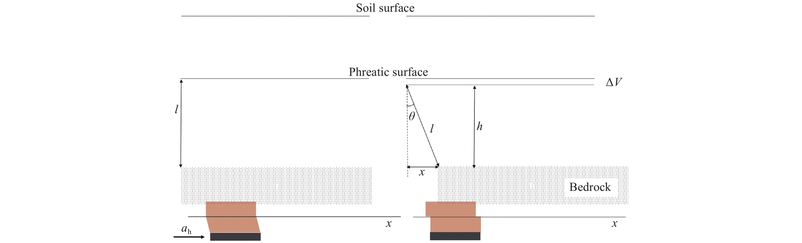
 DownLoad: