Shaotong Wang, Laiyu Lu (2024). On the eigenvalues and eigendisplacement of the critical mode in horizontally layered media. Earthq Sci 37(1): 13-35. DOI: 10.1016/j.eqs.2023.11.005
Citation:
Shaotong Wang, Laiyu Lu (2024). On the eigenvalues and eigendisplacement of the critical mode in horizontally layered media. Earthq Sci 37(1): 13-35. DOI: 10.1016/j.eqs.2023.11.005
Shaotong Wang, Laiyu Lu (2024). On the eigenvalues and eigendisplacement of the critical mode in horizontally layered media. Earthq Sci 37(1): 13-35. DOI: 10.1016/j.eqs.2023.11.005
Citation:
Shaotong Wang, Laiyu Lu (2024). On the eigenvalues and eigendisplacement of the critical mode in horizontally layered media. Earthq Sci 37(1): 13-35. DOI: 10.1016/j.eqs.2023.11.005
• The singularity of critical modes in a horizontally layered medium is investigated when the phase velocity at certain frequency of a mode is equal to the velocity of the P or S wave in a layer.
• A method for calculating the eigendisplacements of these critical modes in the classical transfer matrix method is proposed.
• It is found that the eigendisplacement of the critical mode whose phase velocity equal to S velocity in the bottom half-space remains constant in the bottom half-space, instead of decaying to zero with depth as normal modes.
• An SH critical mode (Love mode) exists in a uniform half-space model with a phase velocity equal to the S velocity, which is similar to the classical Rayleigh mode of P-SV type in the uniform half-space, but the eigenfunction remains constant with depth.
Abstract
Wave propagation in horizontally layered media is a classical problem in seismic-wave theory. In semi-infinite space, a nondispersive Rayleigh wave mode exists, and the eigendisplacement decays exponentially with depth. In a layered model with increasing layer velocity, the phase velocity of the Rayleigh wave varies between the S-wave velocity of the bottom half-space and that of the classical Rayleigh wave propagated in a supposed half-space formed by the parameters of the top layer. If the phase velocity is the same as the P- or S-wave velocity of the layer, which is called the critical mode or critical phase velocity of surface waves, the general solution of the wave equation is not a homogeneous (expressed by trigonometric functions) or inhomogeneous (expressed by exponential functions) plane wave, but one whose amplitude changes linearly with depth (expressed by a linear function). Theories based on a general solution containing only trigonometric or exponential functions do not apply to the critical mode, owing to the singularity at the critical phase velocity. In this study, based on the classical framework of generalized reflection and transmission coefficients, the propagation of surface waves in horizontally layered media was studied by introducing a solution for the linear function at the critical phase velocity. Therefore, the eigenvalues and eigenfunctions of the critical mode can be calculated by solving a singular problem. The eigendisplacement characteristics associated with the critical phase velocity were investigated for different layered models. In contrast to the normal mode, the eigendisplacement associated with the critical phase velocity exhibits different characteristics. If the phase velocity is equal to the S-wave velocity in the bottom half-space, the eigendisplacement remains constant with increasing depth.
Normal mode is an important concept in seismic wave propagation in the Earth (Lapwood and Usami, 1981; Aki and Richards, 2002; Dahlen and Tromp, 1998). For a spherical Earth treated as a finite body, the normal modes describing its fundamental vibration are its free oscillations, forming a complete set of orthogonal functions. By summing these normal modes, it is possible to simulate complete theoretical seismograms (Gilbert, 1971; Maupin, 1996; Yang HY et al., 2010). At regional or local scales, the Earth can be approximated as a horizontally layered model. Body waves excited by seismic sources generate multiple reflections and transmissions in multilayered media. These phenomena can be described in the frequency domain by a set of normal modes. In the P-SV system, these normal modes correspond to Rayleigh waves in the layered medium, whereas in the SH system, they represent Love waves. As their energy is mainly concentrated in the uppermost layers, these normal modes are known as seismic surface waves. The phase velocity of seismic surface waves is highly sensitive to the S-wave velocity of the medium; therefore, the dispersion characteristics of surface waves are widely used for inverting the S-wave velocity structure of the Earth at different scales.
Unlike the spherical Earth, the horizontally layered model is an open system, and the normal modes in this model are not complete, meaning they cannot be used to synthesize complete theoretical seismograms (Maupin, 1996). For instance, in actual seismic records, a dispersive phase called the PL phase exists between the P- and S-waves (Oliver and Major, 1960; Phinney, 1961). This phase is the leaky mode in a layered medium (Chimenti et al., 1982; Haddon, 1984), in which energy can radiate into the underlying half-space medium. The leaky mode can be combined with the normal modes to synthesize the wavefield in a horizontally layered medium (Haddon, 1984, 1986). With the development of dense array observations and seismic interferometry, effective multimode surface wave and leaky mode dispersion curves (Li ZB et al., 2022) can be extracted using data from active sources or ambient noise (e.g., Wang JN et al., 2019; Hu SQ et al., 2020; Qin TW et al., 2022; Qin TW and Lu LY, 2022). The inversion of multimode surface waves can improve the stability and resolution of inversions (Xia JH et al., 2003; Fu L et al., 2022), whereas leaky modes are more sensitive to P-wave velocity. Therefore, the use of multiple normal and/or leaky modes to invert the parameters of the medium has gradually attracted the attention of seismologists (Li ZB et al., 2021; Sun CY et al., 2021; Kennett, 2023).
The normal modes are associated with the real eigenvalues of the dispersion equation. This means that both the frequency and horizontal wavenumber are real. Leaky modes are associated with the complex eigenvalues of the dispersion equation (Haddon, 1984, 1986; Maupin, 1996). A dispersion image is plotted as a function of the real frequency and phase velocity. Modes with phase velocities less than the S-wave velocity in the bottom half-space are referred to as normal modes. The real parts of the eigenvalues for the leaky and normal modes are similar (Shi CW et al., 2022) in this velocity range. Therefore, leaky modes usually refer to modes with phase velocities greater than the S-wave velocity in the bottom half-space.
Eigenvalues and eigenfunctions of the normal and leaky modes in horizontally layered media represent classical problems in seismic wave propagation (Ewing et al., 1957; Brekhovskikh, 1980; Kennett, 1983). The transfer matrix (TM) method is a classical approach to solving such problems (Thomson, 1950; Haskell, 1953). In this method, the matrices described by the parameters of each layer are connected via the continuity conditions at each interface. By applying the radiation conditions to the bottom half-space, the matrix at the surface layer can be obtained by transferring the matrix in the bottom half-space layer-by-layer to the free surface. By applying the boundary conditions at the free surface, a dispersion equation can be obtained using the conditions for nontrivial solutions. Matrix formulation has been improved to avoid the loss of significant digits in numerical computations and simplify the form of the TM (e.g., Thrower, 1965; Dunkin, 1965; Knopoff, 1964; Schwab and Knopoff, 1970; Menke, 1979; Abo-Zena, 1979; Zhang BX et al., 1996). Another method for solving such problems is the generalized reflection and transmission coefficient (GRT) method, originally proposed by Kennett (e.g., Kennett and Kerry, 1979; Kennett, 1983). Luco and Apsel (1983) improved this method. Chen XF (1993) proposed an algorithm using the GRT method to compute eigenvalues and eigenfunctions in horizontally layered media, which avoids exponential growth terms in numerical calculations and exhibits good stability.
The most common process for searching the root of the dispersion equation for normal modes is to search for the real roots of the dispersion equation for a given real frequency. Similarly, for the calculation of leaky modes, the process involves searching for the complex roots of the dispersion equation. The real part of the complex root is plotted in the phase-velocity dispersion image. The S-wave velocity in the bottom half-space serves as the boundary separating the normal and leaky modes. If the phase velocity exceeds the S-wave velocity in the bottom half-space, the dispersion equation has no real roots, and the complex roots are associated with leaky modes. However, a special case should be considered, that is, the case in which the phase velocity equals the P- and S-wave velocities in each layer over the half-space. This case, referred to as the critical phase velocity of the surface waves or the critical mode, should be considered separately because the matrix elements involved in the TM and GRT methods exhibit a singularity.
The conventional root-finding process involves searching for the phase velocity with a certain step size at a given frequency. A velocity within an acceptable error range is considered the root of the dispersion equation. To a large extent, this process avoids the case in which the phase velocity exactly matches the P- and S-wave velocities of the layer over the half-space. Normal modes defined in the frequency domain correspond to multiple reflections and transmissions within each layer of body waves that are incident to the upper interface of the half-space at supercritical angles, whereas leaky modes correspond to waves with an incident angle less than the critical angle. In reality, the critical mode corresponds to the body waves incident at a critical angle. Compared with normal modes, the eigenfunction of the critical mode exhibits specific characteristics. Buchen and Ben-Hador (1996) defined the wave field for the phase velocity to be equal to the body wave velocity of each layer over the half-space; however, a detailed study of the eigenfunction characteristics of the critical mode has not been conducted.
The main purpose of this study was to address the singularity of the critical mode by introducing a general linear solution to the wave equation. The eigenvalues and eigenfunctions of surface waves were calculated based on GRT theory. Using the same theoretical framework as that of the GRT, the singularity of the matrix elements for the critical mode was determined by supplementing the wave field definition at the critical phase velocity. This allowed us to calculate the eigenvalues and eigendisplacements when the phase velocity equaled the body-wave velocity in each layer over the half-space. Furthermore, the characteristics of the eigenvalues and eigendisplacements of the critical modes were analyzed for different horizontally layered models.
2.
GRT method in horizontally layered media
In this section, we review the theory of GRT in horizontally layered media, referring mainly to the theoretical framework and variable representation conventions of Chen XF (1993) and He YF et al. (2006).
2.1
Wave equations and displacement-stress vector
Considering the N+1 horizontally layered medium, as shown in Figure 1, the z-axis was oriented vertically downward and positive. The density, Lamé constants, and shear modulus of the j-th layer are represented by ρ(j), λ(j), and μ(j), respectively. The upper and lower boundaries of the j-th layer are denoted as z(j−1) and z(j). Surface-wave normal modes, as intrinsic properties of horizontally layered media, are nontrivial solutions to source-free elastic dynamic equations subject to boundary conditions (Chen XF, 1993). The two-dimensional source-free elastic dynamic equations governing the motion in each layer are given by
Figure
1.
Horizontal layered model with N+1 layers; the interface depth is marked on the left side of the coordinate axis z, and the layer index, density, and Lamé constant are listed from left to right within the layers.
where j=1,2,⋯,N+1, ⇀u(j) represents the displacement, and ∇ is the Hamiltonian operator.
By performing Fourier transformation and basis function expansion on Equation (1), the differential equations can be obtained for the SH and P-SV systems, respectively:
where u(j) is the eigedisplacement, and τ(j) the eigen stress; they are associated with coefficients obtained by expanding the source-free elastic dynamic equations using basis functions (Zhang HM, 2021). ω is the angular frequency, and k the horizontal wavenumber. Equations (2) and (3) can be written as follows:
where {\boldsymbol{Y}}^{\left(j\right)}\left(z\right) is the displacement-stress vector. The solution {\boldsymbol{Y}}^{\left(j\right)}\left(z\right) of Equation (4) can be written as
The formulation can be re-normalized such that the diagonal matrix has the form {\rm{diag}}[{\varLambda }_{d}^{\left(j\right)}\left(z\right),{\varLambda }_{u}^{\left(j\right)}\left(z\right)]= {\rm{diag}} [{{\rm{e}}}^{-{\nu }^{\left(j\right)}(z-{z}^{\left(j-1\right)})},{{\rm{e}}}^{-{\nu }^{\left(j\right)}({z}^{\left(j\right)}-z)}](Chen XF, 1993). The down- and up-going waves for the SH system can be represented by {[{C}_{d}^{\left(j\right)},{C}_{u}^{\left(j\right)}]}^{{\rm{T}}}={[{\grave{H}}^{\left(j\right)},{\mathop H \limits^{\prime}}{}^{\left(j\right)}]^{{\rm{T}}}}.
For the P-SV system, matrix elements {\boldsymbol{E}}_{mn}^{\left(j\right)}(m,n=\mathrm{1,2}) in Equation (5) can be represented as submatrices of the following 4 × 4 matrix:
where {\rm{diag}}[{\boldsymbol{\varLambda }}_{d}^{\left(j\right)}\left(z\right),{\boldsymbol{\varLambda }}_{u}^{\left(j\right)}\left(z\right)] = {\rm{diag}} [{{\rm{e}}}^{-{\gamma }^{\left(j\right)}\left(z-{z}^{\left(j-1\right)}\right)},{{\rm{e}}}^{{-\nu }^{\left(j\right)}\left(z-{z}^{\left(j-1\right)}\right)}, {{\rm{e}}}^{-{\gamma }^{\left(j\right)}\left({z}^{\left(j\right)}-z\right)},{{\rm{e}}}^{-{\nu }^{\left(j\right)}({z}^{\left(j\right)}-z)}] is a diagonal matrix. {[{\boldsymbol{C}}_{d}^{\left(j\right)},{\boldsymbol{C}}_{u}^{\left(j\right)}]}^{{\rm{T}}}={[{\grave{P}}^{\left(j\right)},{\grave{V}}^{\left(j\right)},{\mathop P \limits^{\prime}}{}^{\left(j\right)},{\mathop V \limits^{\prime}}{}^{\left(j\right)}]^{{\rm{T}}}} is the coefficient of the downward and upward waves. {\alpha }^{\left(j\right)}={\left({{\lambda }^{\left(j\right)}+2{\mu }^{\left(j\right)}}/{{\rho }^{\left(j\right)}}\right)}^{{1}/{2}} is the P-wave velocity, and {\beta }^{\left(j\right)}={\left({{\mu }^{\left(j\right)}}/{{\rho }^{\left(j\right)}}\right)}^{{1}/{2}} is the S-wave velocity. {\gamma }^{\left(j\right)}={\left({k}^{2}-{{\omega }^{2}}/{{{\alpha }^{\left(j\right)}}^{2}}\right)}^{{1}/{2}} and {\nu }^{\left(j\right)}={\left({k}^{2}-{{\omega }^{2}}/{{{\beta }^{\left(j\right)}}^{2}}\right)}^{{1}/{2}}are quantities related to vertical wavenumbers i{\gamma }^{\left(j\right)} and i{\nu }^{\left(j\right)} associated with P- and SV-waves, respectively. i is an imaginary unit. Taking single-valued analytic branches for multi-valued functions on the complex plane requires {\rm{Re}}\left({\nu }^{\left(j\right)}\right)\ge 0 and {\rm{Re}}\left({\gamma }^{\left(j\right)}\right)\ge 0, where {\rm{Re}} denotes the real part. Moreover, if both the real and imaginary parts of {\gamma }^{\left(j\right)} or {\nu }^{\left(j\right)} are equal to zero, Equation (5) exhibits singularities.
2.2
Generalized R/T method
Taking the P-SV system as an example, a set of differential equations governing the up- and down-going waves can be derived based on Equation (5). The continuity conditions of the displacement-stress vector at the interfaces, that is at z={z}^{\left(j\right)} , can be written as
By applying the continuity conditions in Equation (8), the equations satisfying the stress-free surface can be obtained using the transfer matrix. The conditions of the nontrivial solution of these equations lead to the eigenequations of surface waves. Therefore, the matrix in Equation (5) is referred to as the transfer matrix (Gilbert and Backus, 1966; Buchen and Ben-Hador, 1996).
In each layer, there are waves from the upper interface that undergo transmission as down-going waves and waves from the lower interface that undergo reflection as upgoing waves. Chen XF (1993) introduced modified reflection and transmission (R/T) coefficients at arbitrary interfaces. They are {\boldsymbol{R}}_{ud}^{\left(0\right)}, the coefficient at free surface ( j=0 ), the one at the intermediate layers ( j=\mathrm{1,2},\cdots ,N-1 ), denoted as {\boldsymbol{T}}_{d}^{\left(j\right)}, {\boldsymbol{R}}_{ud}^{\left(j\right)}, {\boldsymbol{R}}_{du}^{\left(j\right)}, and {\boldsymbol{T}}_{u}^{\left(j\right)}, and the one at the bottom layer ( j=N ), denoted as {\boldsymbol{T}}_{d}^{\left(N\right)} and {\boldsymbol{R}}_{du}^{\left(N\right)}. These coefficients satisfy:
By applying the continuity and boundary conditions of the zero stresses at the free surface, as well as the radiation boundary condition (no upgoing waves in the half-space) and natural boundary conditions (the displacement and stress are limited at infinite depth), the modified R/T coefficients at the free surface ( j=0 ) can be obtained by
The generalized R/T coefficients can be defined based on the modified R/T coefficients. The generalized R/T coefficients {\widehat{\boldsymbol{T}}}_{d}^{\left(j\right)} and {\widehat{\boldsymbol{R}}}_{du}^{\left(j\right)} for the down-going waves are defined as
where j=\mathrm{1,2},\cdots ,N . The generalized R/T coefficients, {\widehat{\boldsymbol{T}}}_{u}^{\left(j\right)} and {\widehat{\boldsymbol{R}}}_{ud}^{\left(j\right)}, for the upgoing waves are defined as
where j=\mathrm{1,2},\cdots ,N-1 . In the bottom half-space, using the radiation boundary condition, we have {\widehat{\boldsymbol{T}}}_{d}^{\left(N\right)}={\boldsymbol{T}}_{d}^{\left(N\right)} and {\widehat{\boldsymbol{R}}}_{du}^{\left(N\right)}={\boldsymbol{R}}_{du}^{\left(N\right)}. At the free surface, the generalized reflection coefficient {\widehat{\boldsymbol{R}}}_{ud}^{\left(0\right)} can be obtained using the free-surface boundary condition, which satisfies {\boldsymbol{C}}_{d}^{\left(1\right)}={\widehat{\boldsymbol{R}}}_{ud}^{\left(0\right)}{\boldsymbol{C}}_{u}^{\left(1\right)}.
By substituting Equation (13) into Equation (9), the following recursive relations of the generalized R/T coefficients for downgoing waves can be obtained:
where j=N-1,N-2,\cdots ,1 . For j=N , we have {\widehat{\boldsymbol{T}}}_{d}^{\left(N\right)}={\boldsymbol{T}}_{d}^{\left(N\right)} and {\widehat{\boldsymbol{R}}}_{du}^{\left(N\right)}={\boldsymbol{R}}_{du}^{\left(N\right)}. Based on the coefficients in the bottom half-space, the generalized R/T coefficients at the top layer can be obtained using Equation (15).
Similarly, by substituting Equation (14) into Equation (9), the recursive relations of the generalized R/T coefficients for the upgoing waves can be obtained:
where j=\mathrm{1,2},\cdots ,N . For j=0 , we have {\widehat{\boldsymbol{R}}}_{ud}^{\left(0\right)}={\boldsymbol{R}}_{ud}^{\left(0\right)}. The generalized R/T coefficients in the bottom half-space can be obtained using Equation (16).
The modified R/T coefficients for each layer can be calculated using Equation (11), and the generalized R/T coefficients can be obtained using Equations (15) and (16). According to Pei D et al. (2008), generalized R/T coefficients can be directly defined without defining modified R/T coefficients. Because the modified R/T coefficients include vertical phase delays and provide information on the reflection and transmission at each interface, they provide a clearer and more physical explanation of the wave function of the critical phase velocity. We began by defining the modified R/T coefficients and embedding the wave function related to the critical phase velocity into them.
2.3
Dispersion equation
Similar to the transfer matrix method, the eigenequation can be derived using recursive relations and zero free-surface stresses:
In theory, the dispersion equation shown in Equation (17) encompasses all eigenvalues of the normal modes. However, missing roots may occur in practical calculations, particularly when low-velocity layers are present. To address this issue, He YF et al. (2006) proposed the concept of a secular function family, building on Chen XF (1993).
For down-going wave coefficient {\boldsymbol{C}}_{d}^{\left(j\right)} to be a nonzero solution, the determinant of the coefficient matrix in Equation (19) must equal zero:
The left side of Equation (20) is referred to as the secular function family (Chen XF, 1993; He YF et al., 2006; Wu B, 2016). Chen XF (1993) initially derived the eigenequation of surface waves using the generalized R/T coefficients in the first layer, that is, when j=1 in Equation (19).
In Equation (20), the secular function associated with each layer j leads to an eigenequation. Theoretically, these equations are equivalent. By considering the sensitivity of the surface wave modes to the depths, the secular functions can be selected at the appropriate layer to avoid missing the root caused by the numerical calculation used to find the eigenvalue. Wu B and Chen XF (2016) proposed an adaptive method for selecting the secular functions. After obtaining the eigenvalues of the surface waves using Equation (20), they can be substituted into Equation (18) to compute the coefficients of the up- and down-going waves. The eigenfunctions of the different surface-wave modes can then be calculated using Equation (5).
3.
Theory and methods
Based on the generalized R/T coefficients and considering the secular function family for either the free surface or an appropriate layer, the eigenvalues and eigenfunctions of the surface waves can be effectively calculated by decreasing the overflow at high frequencies (He YF et al., 2006; Wu B and Chen XF, 2016). To determine the phase velocity of the surface waves, a specific frequency is provided, and the phase velocities for different modes are searched in steps by solving the root of the eigenequation. Once the searched velocity satisfies the error requirements, it is considered the phase velocity at a given frequency. From the numerical computation, a situation in which the searched phase velocity exactly matches the P- or S-wave velocity of the layer is largely avoided during this process. Another scheme for determining the eigenvalue is to identify the frequency of a given phase velocity. In this case, the given phase velocity may exactly matches the P- or S-wave velocity of the layer, that is, the critical phase velocity of the surface wave or critical mode. The matrix formulation presented in Section 2.1 does not define the critical mode well. Although the critical phase velocity satisfies {\rm{Re}}\left({\nu }^{\left(j\right)}\right)\ge 0 and {\rm{Re}}\left({\gamma }^{\left(j\right)}\right)\ge 0\ge 0, if {\nu }^{\left(j\right)}=0 or {\gamma }^{\left(j\right)}=0 , both the real and imaginary parts of {\gamma }^{\left(j\right)} or {\nu }^{\left(j\right)} are zero, leading to the singularity in Equation (5).
Owing to the reciprocal relationship between the ray parameter and phase velocity, the critical phase velocity corresponds to the critical refraction. Brekhovskikh (1980) discussed the calculation of critical refraction when solving for reflected waves using integral transform methods and obtained a solution for the primary reflection wave (corresponding to a ray path). In the frequency domain, the surface wave field is a superposition of an infinite number of modes (Harkrider, 1964; Saito, 1967). In the time domain, this corresponds to a combination of infinite body-wave rays (Wigginst and Helmberger, 1974; Cerveny, 1979; Zhao L and Dahlen, 1996). Investigating the eigenvalues and eigenfunctions of surface waves at the critical phase velocity aids our understanding of the relationship between modes and rays for the surface wave field, particularly the energy distribution for critical refraction. Starting from the general solution of the wave equation, we studied the reasons for the singularity of the matrix formulation at the critical phase velocity of surface waves. A solution to overcome this singularity was proposed. Moreover, the characteristics of the critical mode eigenfunctions were investigated for different layered models.
3.1
Fundamental solution of the wave equation
For simplicity, the superscript omits the index of the layer. In each layer, the wave equations of the SH-wave displacement and the P- and SV-wave potential functions can be written as
where {u}_{y} is the SH-wave displacement, \varphi is the P-wave potential function, and \psi is the SV-wave potential function. Equation (21) is solved by the separation of variables. Taking the equation of SH-wave displacement as an example:
where {k}_{z}={\left({{\omega }^{2}}/{{\beta }^{2}}-{k}^{2}\right)}^{{1}/{2}},\;{\rm{Re}}\left({k}_{z}\right)\ge 0. \omega is the angular frequency, k is the horizontal wavenumber, and {k}_{z} is the vertical wavenumber. Because the eigenfunctions of surface waves in horizontally layered media depend only on depth z , only the solution of the differential equation related to {k}_{z} was considered.
Three general solutions can be obtained for the differential equation in Equation (23). When {k}_{z} is a nonzero real number, the general solution is given by:
where {C}_{1} and {C}_{2} are the arbitrary constants. The trigonometric functions in Equation (24) represent a homogeneous plane-wave solution with a real incident angle.
When {k}_{z} is purely imaginary and has a positive imaginary component, the general solution is given by
Equation (25) represents the waves that increase or decrease exponentially with depth. This is an inhomogeneous plane wave with a complex incident angle.
When {k}_{z} is zero, the general solution is given by
Z\left(z\right)={C}_{1}+{C}_{2}z.
(26)
Equation (26) represents a plane wave propagating along the horizontal plane, and its amplitude varies linearly with depth.
Equations (24) and (25) can be written in a unified form as
Z\left(z\right)=\grave{C}{{\rm{e}}}^{{\rm{i}}{k}_{z}z}+{\mathop C \limits^{\prime}} {{\rm{e}}}^{-{\rm{i}}{k}_{z}z}.
(27)
The general solutions of the potential functions \varphi and \psi in Equation (21) are similar to Equations (26) and (27) with {k}_{z}={\left({{\omega }^{2}}/{{\alpha }^{2}}-{k}^{2}\right)}^{{1}/{2}} for \varphi . Equation (27) represents the downward or upward propagating homogeneous plane wave for a real nonzero {k}_{z} . If {k}_{z} is purely imaginary and has a positive imaginary part, Equation (27) represents an evanescent or inhomogeneous plane wave, corresponding to either the downward or upward tunneling phenomenon (Mellman and Helmberger, 1974; Brekhovskikh, 1980). The solution given by Equation (27) is equivalent to the plane-wave solutions of Equation (5), whereas the linear solution described by Equation (26) is ignored in Equation (5). The existence of this solution requires {k}_{z} to be zero, leading to critical modes, which can be interpreted as the modes in which phase velocity c equals the P- or S-wave velocity of the layer above the half-space. This critical mode was described by Ewing et al. (1957) to account for grazing incidence phenomena. Compared with Equation (27), a clear feature of Equation (26) is its independence from the frequency.
To avoid the singularity arising in Equation (5) when the phase velocity equals the P- or S-wave velocity of each layer and calculate the eigenvalues and eigenfunctions of the critical mode within the existing theoretical framework, the linear solution presented in Equation (26) can be embedded into the generalized R/T coefficients. For this purpose, we define term {C}_{1} in Equation (26) as the “down-going wave” and term {C}_{2}z as the “up-going wave”. Equation (26) can be rewritten as
Z\left(z\right)=\grave{C}+{\mathop C \limits^{\prime}}z.
(28)
In addition, to satisfy the natural boundary condition in the bottom half-space, we set {\mathop C \limits^{\prime}}=0. The down-going waves in the bottom half-space, such as the downward homogeneous, inhomogeneous, and constant plane waves, propagate downward without generating any “reflected” waves from the bottom half-space. In this study, the boundary conditions in the half-space that must be satisfied are referred to as radiation conditions. The downward propagating homogeneous plane wave corresponds to the leaky mode related to the refraction of the half-space interface at angles less than the critical angle. The downward inhomogeneous plane wave corresponds to the normal mode related to the refraction at angles greater than the critical angle. The downward constant plane wave corresponds to critical refraction, which is the boundary between the normal and leaky modes.
Equation (28) can be rewritten as
\grave{C}+{\mathop C \limits^{\prime}} z\to \grave{C}+{\mathop C \limits^{\prime}}\left(z-{z}^{\left(s-1\right)}\right),
(29)
where s\in \mathrm{1,2},\cdots ,N . By comparing the displacement-stress vector obtained from the solutions of Equations (27) and (29) with the general solution of Equation (5), the singularity of the critical mode can be addressed by modifying the matrix formulation.
3.2
Transfer matrix formulation at the critical phase velocity
3.2.1
SH system
For the SH system, the solution of the wave equation in Equation (21) is consistent with the eigen displacement-stress vector in Equation (5). The matrix formulation of the critical mode can be directly obtained based on the general solution shown in Equation (29).
If phase velocity c={\beta }^{\left(s\right)} ( s is the index of layers from \mathrm{1,2},\cdots ,N+1 ), the eigen displacement-stress vector in the s -th layer can be expressed as
\left\{\begin{array}{l}{u}_{y}^{\left(s\right)}\left(z\right)={\grave{H}}^{\left(s\right)}+{{\mathop H \limits^{\prime}}{}^{\left(s\right)}}\left(z-{z}^{\left(s-1\right)}\right)\\ {\tau }_{zy}^{\left(s\right)}\left(z\right)={\mu }^{\left(s\right)}{{\mathop H \limits^{\prime}}{}^{\left(s\right)}}\end{array}\right..
(30)
The transfer matrix occurred in Equation (5) for c={\beta }^{\left(s\right)} is then given by
The diagonal matrix is {\rm{diag}}[{\varLambda }_{d}^{\left(s\right)}\left(z\right),{\varLambda }_{u}^{\left(s\right)}\left(z\right)]={\rm{diag}} \left[\mathrm{1,1}\right]. The coefficients of the down- and up-going waves are {[{C}_{d}^{\left(s\right)},{C}_{u}^{\left(s\right)}]^{{\rm{T}}}}={[{\grave{H}}^{\left(s\right)},{{\mathop H \limits^{\prime}}{}^{\left(s\right)}}]^{{\rm{T}}}}. Considering the radiation conditions in half-space, {{\mathop H \limits^{\prime}}{}^{\left({\rm{N}}+1\right)}}=0 for s=N+1 . The transfer matrices for the other layers remain, except for the s -th layer, where the phase velocity is equal to the body-wave velocity.
3.2.2
P-SV system
For the P-SV system, the solution given by Equation (29) represents the solution of the potential function. The displacement-stress vector obtained by the potential functions using Hooke’s law differs from that in Equation (5). Therefore, we redefine the displacement-stress vector as well as the coefficients of down- and upgoing waves as:
where the diagonal matrix is {\rm{diag}}[{\boldsymbol{\varLambda }}_{d}^{\left(s\right)}\left(z\right),{\boldsymbol{\varLambda }}_{u}^{\left(s\right)}\left(z\right)]={\rm{diag}} [{{\rm{e}}}^{-{\gamma }^{\left(s\right)}(z-{z}^{\left(s-1\right)})},1,{{\rm{e}}}^{-{\gamma }^{\left(s\right)}({z}^{\left(s\right)}-z)},1]. The coefficients of the up- and down-going waves are {[{\boldsymbol{C}}_{d}^{\left(s\right)},{\boldsymbol{C}}_{u}^{\left(s\right)}]^{{\rm{T}}}}={[{\grave{\bar{P}}^{\left(s\right)}},{\grave{\bar{V}}^{\left(s\right)}},{{\mathop {\bar P} \limits^{\;\;\prime}}{}^{\left(s\right)}},{{\mathop {\bar V} \limits^{\;\;\prime}}{}^{\left(s\right)}}]^{{\rm{T}}}}.
For c={\alpha }^{\left(s\right)} , the matrix formulation at the s -th layer is:
where the diagonal matrix is {\rm{diag}}[{\boldsymbol{\varLambda }}_{d}^{\left(s\right)}\left(z\right),{\boldsymbol{\varLambda }}_{u}^{\left(s\right)}\left(z\right)]={\rm{diag}} [1,{{\rm{e}}}^{{-\nu }^{\left(s\right)}(z-{z}^{\left(s-1\right)})},1,{{\rm{e}}}^{-{\nu }^{\left(s\right)}({z}^{\left(s\right)}-z)}]. The coefficients of the up- and down-going waves are {[{\boldsymbol{C}}_{d}^{\left(s\right)},{\boldsymbol{C}}_{u}^{\left(s\right)}]}^{{\rm{T}}}={[{\grave{\bar{P}}^{\left(s\right)}},{\grave{\bar{V}}^{\left(s\right)}},{{\mathop {\bar P} \limits^{\;\;\prime}}{}^{\left(s\right)}},{{\mathop {\bar V} \limits^{\;\;\prime}}{}^{\left(s\right)}}]^{{\rm{T}}}}.
Considering the radiation condition in the half-space, {[{{\mathop {\bar P} \limits^{\;\;\prime}}{}^{\left(s\right)}},{{\mathop {\bar V} \limits^{\;\;\prime}}{}^{\left(s\right)}}]^{{\rm{T}}}}={[0,0]}^{{\rm{T}}} for s=N+1 . The transfer matrices for the other layers remained the same, except for the s -th layer. All calculations are the same as those in the original theoretical frame, except the matrix elements are replaced with new ones above the s -th layer. A specific case concerns a multilayered SH system at s=1 . In this case, the definitions of the down- and up-going waves in Equation (26) should be {u}_{y}^{\left(1\right)}\left(z\right)={{\mathop H \limits^{\prime}}{}^{\left(1\right)}}+{\grave{H}^{\left(1\right)}}z, that is, {\mathop H \limits^{\prime}} is now the up-going wave, whereas \grave{H}z is the down-going wave. In this manner, the wave field satisfies the boundary conditions at the free surface and the radiation conditions at infinity in half-space. If we use the definition where {\mathop H \limits^{\prime}}z represents the upgoing wave and \grave{H} represents the downgoing wave, the reflection coefficient at the free surface becomes infinite. Redefining constant {{\mathop H \limits^{\prime}}{}^{\left(1\right)}} as an upgoing wave naturally implies that the energy in the second layer is critically refracted into the first layer when s=1 , generating a constant plane wave that propagates upward in the first layer. Meanwhile, {\grave{H}}^{\left(1\right)}z is zero in this case. There are no waves “reflected” back, and the free surface effectively acts as a half-space.
4.
Numerical simulation
Based on the previous theoretical analysis, numerical simulations were conducted to investigate the eigenvalues and eigenfunctions of the surface waves of the critical mode for different models. The model parameters are listed in Table 1 and include a homogeneous half-space, two velocity-increasing models, and a layered model with a low-velocity layer. The last two columns in Table 1 provide the phase velocity of the classical nondispersive Rayleigh wave mode propagating in a semi-infinite medium, as described by the layer parameters and Poisson’s ratio.
Table
1.
Parameters of the horizontally layered model
For simplicity, the density of each layer is set to 1 g/cm3 and the layer thickness to 5 km. To determine the eigenvalues of the general normal modes from the eigenequation, the phase velocity is searched for a given frequency. For the critical mode, the frequency was searched at a given critical phase velocity. At a frequency range of 0–0.2 Hz, the eigenvalues are calculated at sampling points which are distributed at equal intervals of the phase velocity because it exhibits a large gradient at this frequency range. For frequencies greater than 0.2 Hz, the eigenvalues are calculated at frequencies with equal intervals.
4.1
Critical SH wave in a homogeneous half-space
Model 1 was a homogeneous half-space model. According to the classical wave theory, Love waves exist in a layered model with at least one finite-thickness covering layer. The classical Love wave mode does not exist for a homogeneous half-space model because the theory only considers the general solution from Equation (27). Applying the free-surface boundary condition and radiation condition in the half-space, we immediately obtain coefficients of zero for both up- and down-going waves based on the solution for Equation (27), implying that there are no meaningful solutions for SH systems in a half-space. However, if we consider the solution of the linear function in Equation (29) at c={\beta }^{\left(1\right)} , a meaningful solution for this mode can be obtained. If s=1 in Equation (30), the displacement-stress vector in a homogeneous half-space model can be obtained as:
\left\{\begin{array}{l}{u}_{y}^{\left(1\right)}\left(z\right)={\grave{H}}^{\left(1\right)}+{{\mathop H \limits^{\prime}}{}^{\left(1\right)}}\left(z-{z}^{\left(0\right)}\right)\\ {\tau }_{zy}^{\left(1\right)}\left(z\right)={\mu }^{\left(1\right)}{{\mathop H \limits^{\prime}}{}^{\left(1\right)}}\end{array}\right..
(35)
By applying the free-surface boundary and radiation conditions, we obtained {{\mathop H \limits^{\prime}}{}^{\left(1\right)}}=0. Therefore, a nondispersive but meaningful solution can be obtained. The displacement-stress vector is given by
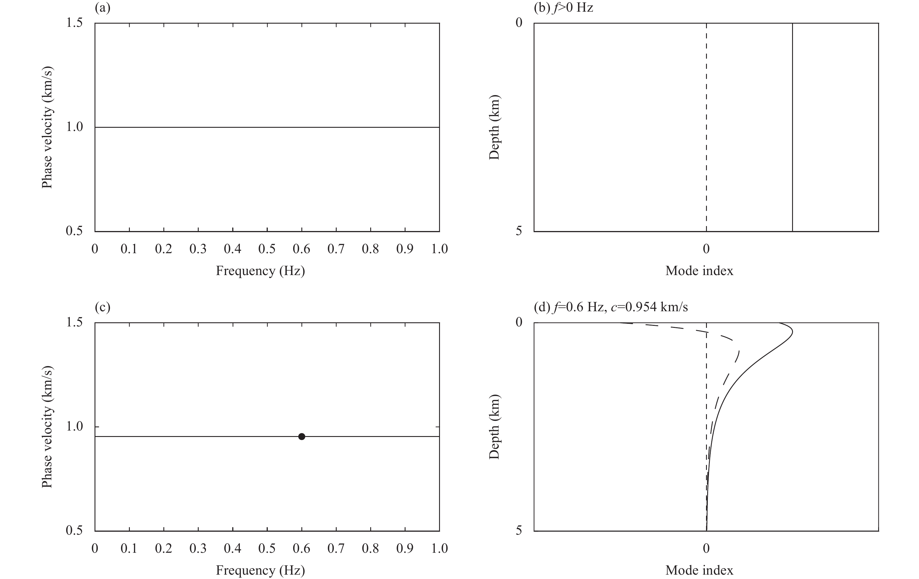
This solution is the critical SH mode in a homogeneous half-space. The eigendisplacement was constant and did not vary with depth. The eigenstress was zero at all depths. Figure 2a and b shows the phase velocity and eigendisplacement of this mode, respectively. The velocity of this mode did not vary with frequency. It propagates horizontally at a velocity equal to the S-wave velocity of the half-space and behaves as a nonattenuating homogeneous plane wave in the vertical direction (Brekhovskikh, 1980). For frequencies greater than zero, the displacement remains constant with depth.
Figure
2.
Eigenvalues and eigendisplacement of Model 1. (a) Phase velocity of the SH critical mode. (b) Eigendisplacement (solid line) of the SH critical mode. (c) Phase velocity of the P-SV system (classic Rayleigh mode). (d) Eigendisplacement of a Rayleigh wave at 0.6 Hz. The solid line denotes the vertical component while the dashed line denotes the horizontal component (the same applies to the following figures). They are normalized by the maximum. The vertical dashed line in (b) and (d) denotes the zero in the horizontal axis.
For the P-SV system, the only normal mode that exists in the half-space is the classical Rayleigh wave, which is formed by the interaction of inhomogeneous P and SV waves at the free surface. For comparison with the SH critical mode, Figure 2c and d shows the eigenvalues and eigendisplacement of the classical Rayleigh wave in Model 1. As is already known, this mode is nondispersive, and the phase velocity is slightly lower than the S-wave velocity of the half-space. The eigendisplacement decayed exponentially with depth. The critical mode does not exist in the homogeneous half-space of the P-SV system.
4.2
Eigenvalues and eigenfunctions of the critical mode in the model with increasing layer velocity
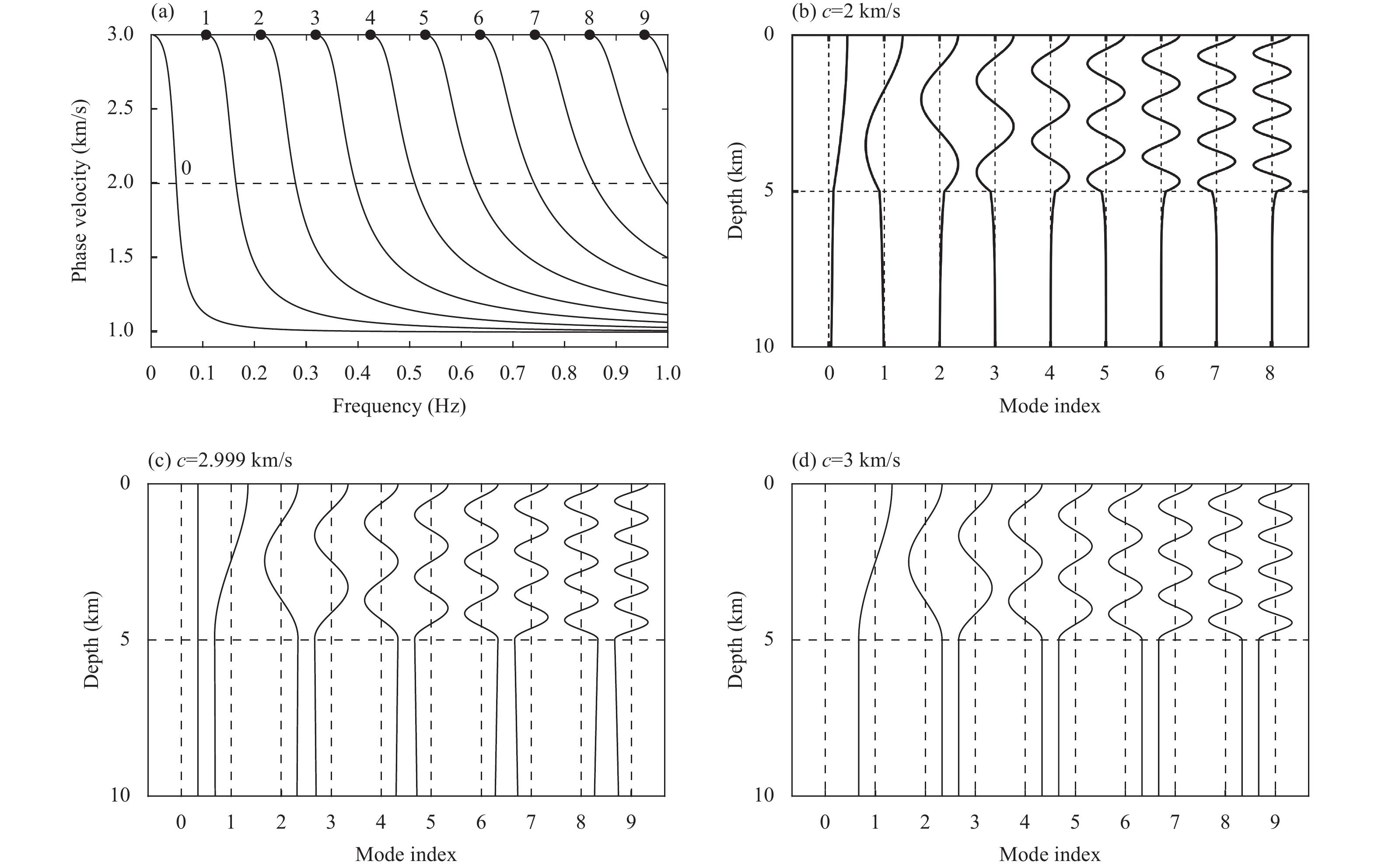
The velocity of the layer in Models 2 and 3 increased with depth. Models 2 and 3 consisted of two and three layers, respectively. Figure 3a shows the phase velocity normal modes of the SH wave in Model 2, which are typical Love waves. The phase velocity of the Love wave modes varies between the S-wave velocity of the first layer and the bottom half-space, i.e., 1\;\mathrm{k}\mathrm{m}/\mathrm{s} < c\le 3\;\mathrm{k}\mathrm{m}/\mathrm{s}. The phase velocity of the fundamental mode tends toward the S-wave velocity of the first layer at high frequencies, i.e., 1\mathrm{ }\mathrm{ }\mathrm{ }\mathrm{ }\mathrm{k}\mathrm{m}/\mathrm{s} . As discussed in Section 4.1, this velocity limit is also a critical SH mode in Model 1, which is a homogeneous half-space model. This is analogous to the Rayleigh wave in layered media, where the high-frequency limit of the phase velocity of the fundamental Rayleigh mode tends toward the phase velocity of the classical Rayleigh wave mode, treating the top layer as a half-space.
Figure
3.
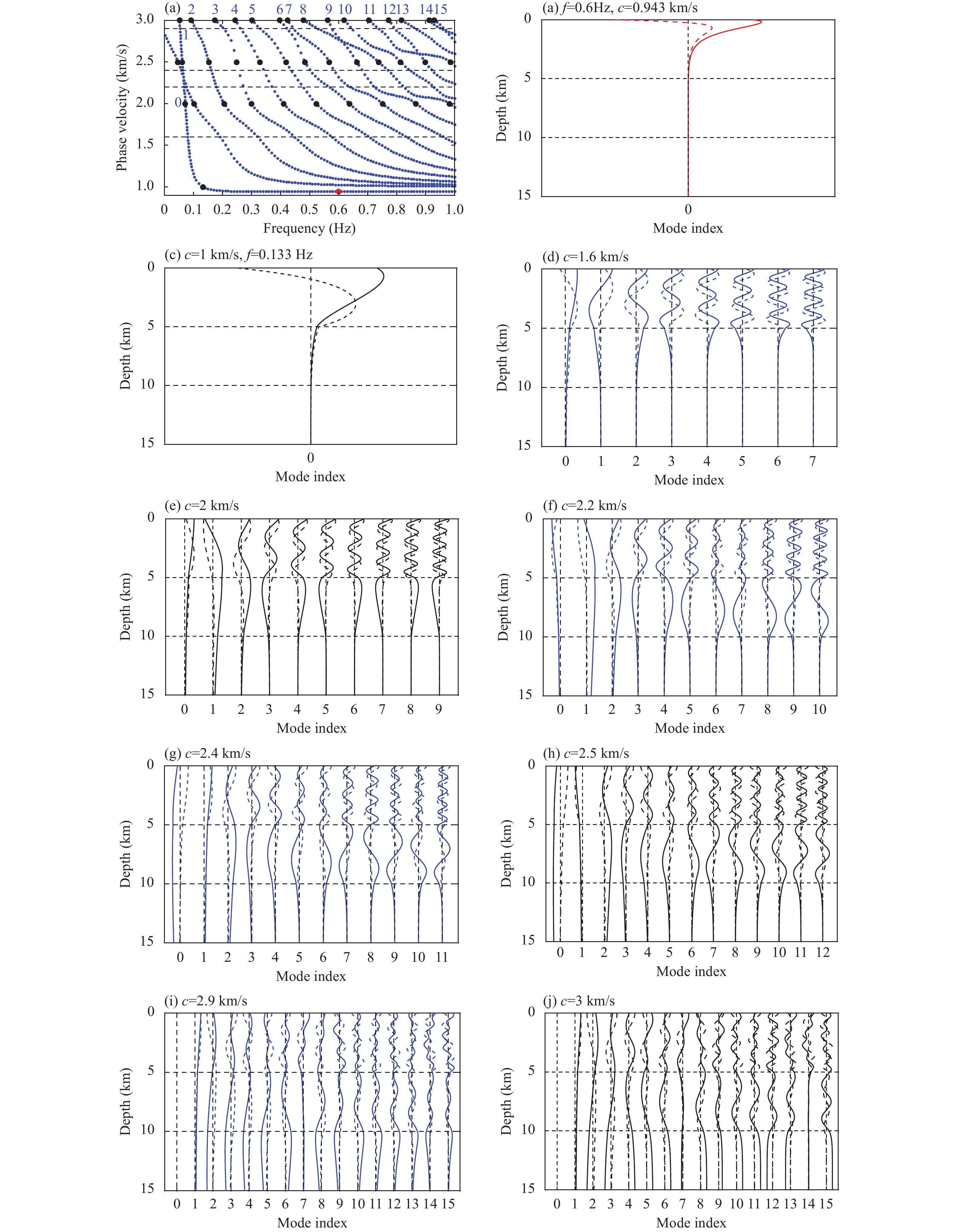
Eigenvalues and eigendisplacement of SH wave in Model 2. (a) Phase velocity of Love waves. The mode indices are labeled in the panel, and the dots represent the critical modes at a phase velocity of 3 km/s. (b) Eigendisplacement as a function of depth at a phase velocity of 2 km/s. The labels of the horizontal axis are the indices of the modes, the vertical dashed lines represent their zero positions. (c) Same as (b) but at 2.999 km/s, close to the critical phase velocity of 3 km/s, i.e., the S-wave velocity in the half-space. (d) Eigendisplacement of the critical mode at 3 km/s, i.e., the eigendisplacement associated with the eigenvalues denoted by dots in (a).
Figure 3b shows the eigendisplacements as a function of the depth at phase velocity c=2\;\mathrm{k}\mathrm{m}/\mathrm{s} , that is, the eigendisplacement associated with the eigenvalues located at the intersections between the black dashed line and the dispersion branches in Figure 3a. Figure 3c shows the eigendisplacements at a phase velocity of c=2.999\;\mathrm{k}\mathrm{m}/\mathrm{s}. Figure 3b and c presents the typical characteristics of eigendisplacements for the phase velocity in the range of 1\;\mathrm{k}\mathrm{m}/\mathrm{s} < c\le 3\;\mathrm{k}\mathrm{m}/\mathrm{s}. The energy is predominantly concentrated in the first layer, corresponding to standing waves in the spatial domain formed by the interference between the upward and downward homogeneous plane waves in the first layer. In this velocity range, these modes are SH-guided waves, where the SH-waves undergo supercritical reflection and transmission at the bottom interface of the first layer (z=5\;\mathrm{k}\mathrm{m}), and the energy is trapped within this layer. In the lower half-space, the eigendisplacements decayed exponentially with depth.
In Figure 3a, the critical modes are referred to as cutoff modes because they correspond to the cutoff frequencies of normal modes. These critical modes indicate the boundaries between the normal and leaky modes. Figure 3d shows the eigendisplacements of these modes. Unlike the normal modes for a phase velocity in the range of 1\;\mathrm{k}\mathrm{m}/\mathrm{s} < c < 3\;\mathrm{k}\mathrm{m}/\mathrm{s}, the eigendisplacements of the critical modes remain constant in the bottom half-space, sharing the same ray parameters (or horizontal slowness) as critically refracted or head waves (Červený and Ravindra, 1971). Their eigendisplacements are closely related to the energy distribution of the critical refracted waves. Comparing Figure 3c and d, the eigendisplacements near the critical phase velocity (2.99 km/s) exhibited continuity with those of the critical modes. In other words, as the phase velocity gradually increases from 1 km/s to a critical velocity of 3 km/s, the decay of the eigendisplacements in the half-space gradually slows until the phase velocity matches the half-space S-wave velocity, and the eigendisplacements are constant in the bottom half-space.
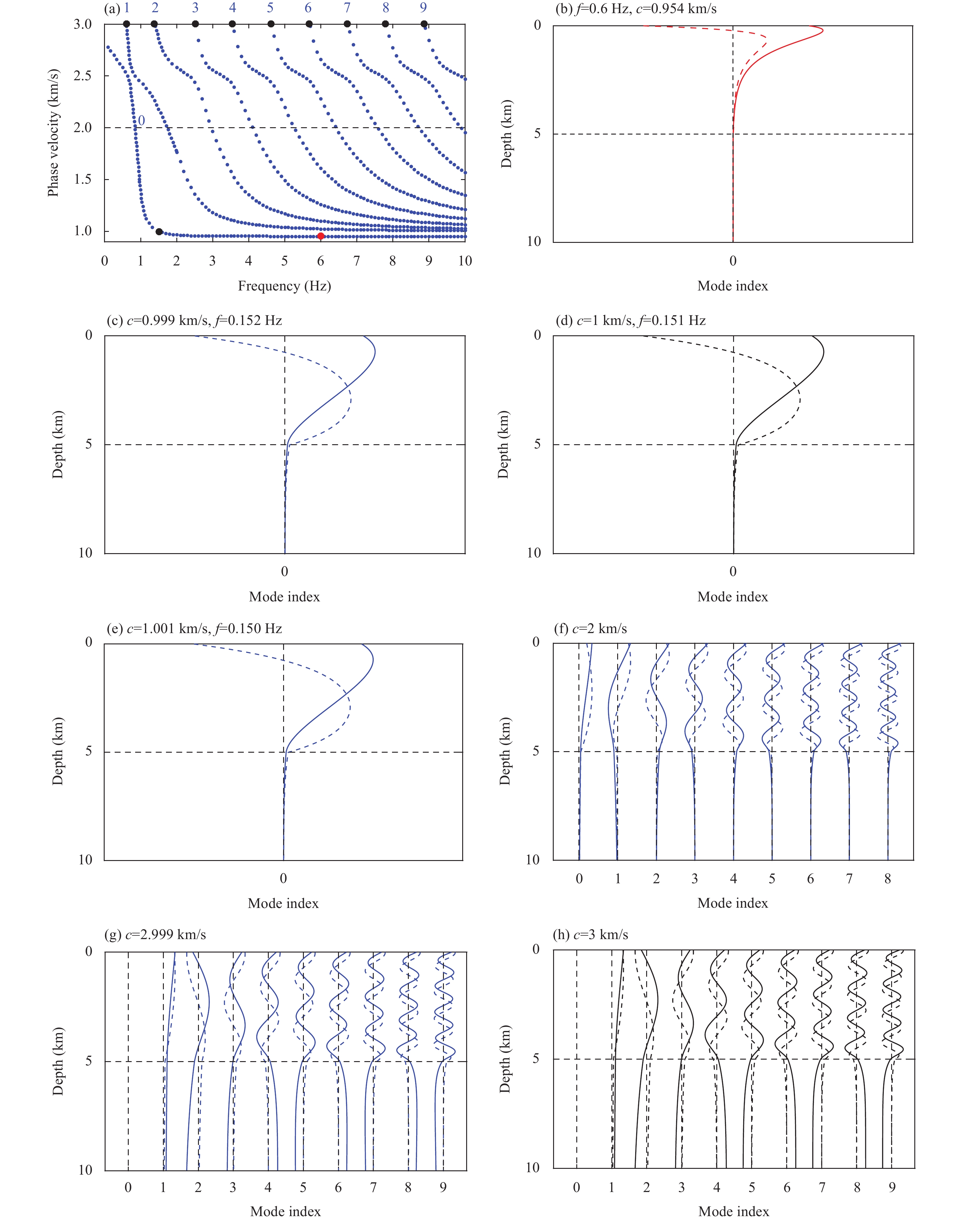
Figure 4 shows the eigenvalues and eigendisplacements of the P-SV wave in Model 2. Compared with the SH system, the clear difference in the P-SV system lies in the fundamental mode. The fundamental Rayleigh mode is caused by the interaction between inhomogeneous P and SV waves at the free surface. At high frequencies, the phase velocity of this mode converges to that (0.954 km/s) of the classic Rayleigh wave in a model formed by treating the first layer as a half-space. At low frequencies, the phase velocity of the mode converges to that of the classic Rayleigh wave (2.834 km/s) in a half-space model without the first layer (Zhang BX and Lu LY, 2002). Bounded by the phase velocity (c=1\;\mathrm{k}\mathrm{m}/\mathrm{s}) of the critical mode, the fundamental Rayleigh wave can be divided into two segments. For segment c<1 km/s, the waves behaved as inhomogeneous plane waves in both the first layer and half-space. For segment c>1 km/s, the waves in the first layer become homogeneous plane waves. The eigendisplacements decayed exponentially with depth for the entire fundamental mode. As the frequency decreased, the decay slowed and the penetration depth increased.
Figure
4.
Eigenvalues and eigendisplacement of P-SV wave in Model 2. (a) Phase velocity of Rayleigh waves. (b) Eigendisplacement associated with the eigenvalues denoted by red dots in (a), where the frequency is 0.6 Hz and phase velocity is 0.954 km/s. (c)–(e) are the eigendisplacement of the fundamental mode at phase velocities of 0.999, 1, and 1.001 km/s, respectively. (f)–(h) are the eigendisplacements of modes at phase velocities of 2, 2.999, and 3 km/s, respectively. In the panels depicting eigendisplacement, blue denotes the normal mode, whereas black denotes the critical mode (the same applies to the following figures).
Similar to the SH modes, high-order P-SV modes with phase velocities ranging from 1\;\mathrm{m}/\mathrm{s} < c < 3\;\mathrm{k}\mathrm{m}/\mathrm{s} are trapped waves (or guided waves) (Zhang BX and Lu LY, 2002). These modes result from the supercritical reflection and transmission of the SV wave and are referred to as SV-type Love waves by Kennett (1983). A comparison of Figures 3b and 4f show that the distributions of the eigendisplacements for the SH and P-SV waves at c=2\;\mathrm{k}\mathrm{m}/\mathrm{s} are similar.
As shown in Figure 4h, the vertical displacements of the critical mode at c=3\;\mathrm{k}\mathrm{m}/\mathrm{s} rapidly approached a constant value in the bottom half-space, whereas the horizontal displacement decayed exponentially with depth. This is similar to the energy distribution of the head wave due to the critical refraction of the SV wave. Figure 4g shows the eigendisplacement at c=2.999\;\mathrm{k}\mathrm{m}/\mathrm{s}, which is close to the phase velocity (3 km/s) of the critical mode.
Owing to slow attenuation with depth, the vertical eigendisplacement in the half-space also appears to approach a constant. Wu B (2016) found this feature for the mode near the critical phase velocity and interpreted it as the radiation mode (Maupin, 1996). This may be caused by the slow decay of the eigendisplacement as it approaches the critical mode. At a sufficiently large depth, the eigendisplacement decays to zero. Conversely, it shows that the variation in the eigendisplacement is continuous from normal to critical mode and proves that the critical mode calculation in this study is reliable.
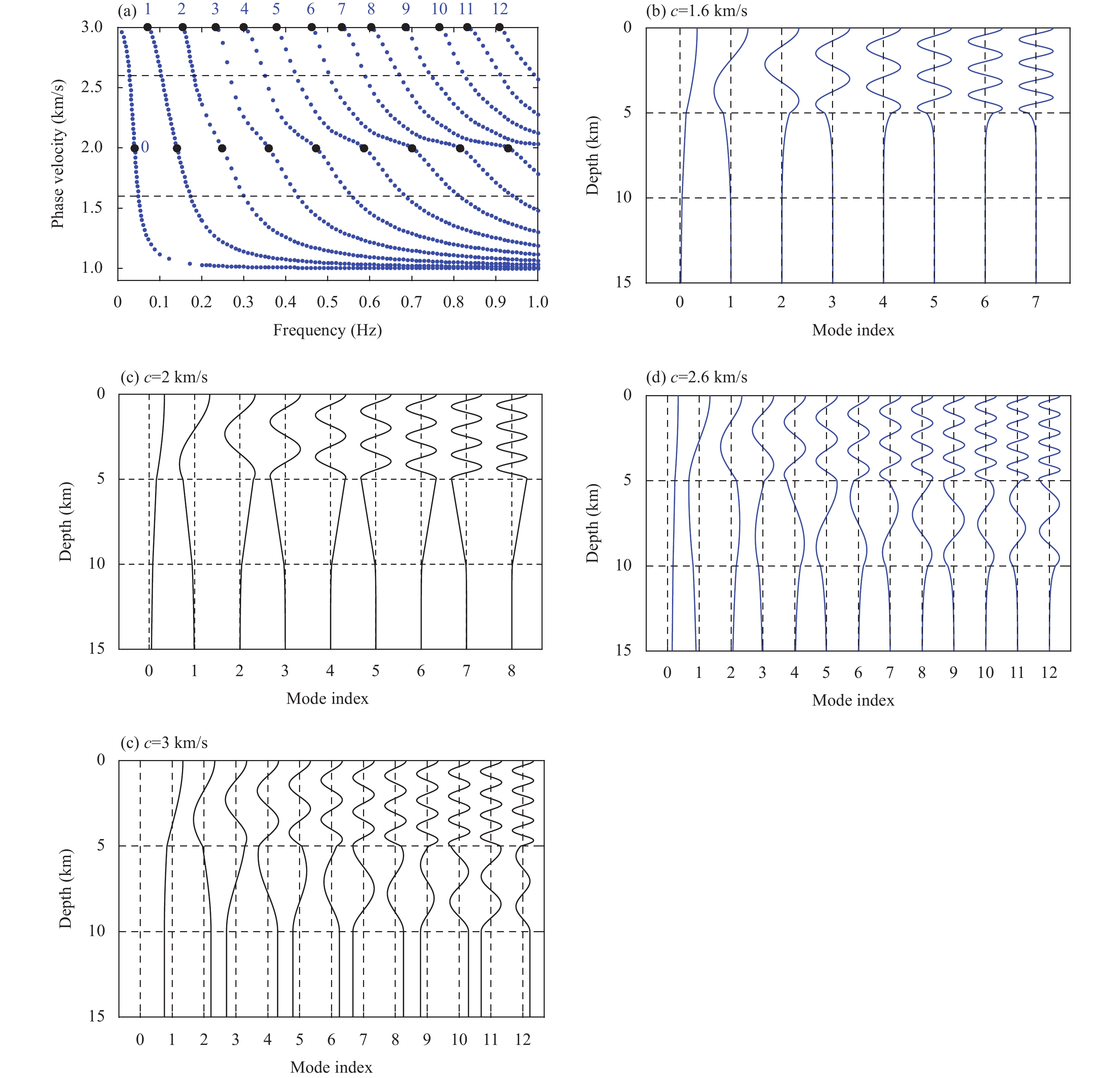
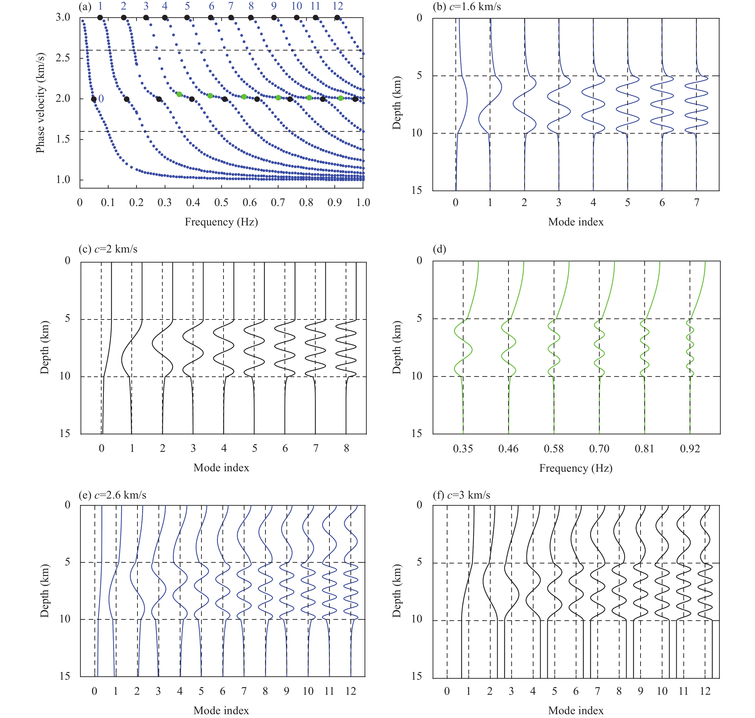
Figure 5 shows the eigenvalues and eigendisplacements of the SH waves in Model 3. Bounded by the S-wave velocities of each layer, the characteristics of the eigendisplacement are determined for modes located in different phase velocity ranges, as performed by Fan YH et al. (2007). If phase velocity c lies between the S-wave velocities of the first layer and bottom half-space, that is, 1\;\mathrm{k}\mathrm{m}/\mathrm{s} < c < 2\;\mathrm{k}\mathrm{m}/\mathrm{s}, the modes exhibit typical normal mode characteristics. Because of the reflection at z=5\;\mathrm{k}\mathrm{m}, most of the energy was concentrated in the first layer. Only a small value is transmitted below the second layer. We selected the eigendisplacement at c=1.6\;\mathrm{k}\mathrm{m}/\mathrm{s} as an example of a normal mode. As shown in Figure 5b, most of the energy is concentrated in the first layer. The eigendisplacement decayed exponentially starting from z=5\;\mathrm{k}\mathrm{m}, the bottom interface of the first layer. In the low-frequency range (e.g., the segment at low frequency for the same dispersion branch or the lower order of modes for the same phase velocity shown in Figure 5b), the eigendisplacement in the half-space decays slowly and has a deep penetration depth, which is well known in surface wave imaging. This is related to the tunneling effect of inhomogeneous waves (Mellman and Helmberger, 1974; Brekhovskikh, 1980) or finite-frequency effects. The inhomogeneous down-going waves in the second layer did not decay to a sufficiently small value at z=10 km, and a small amount of energy was reflected from the interface to the top layers as upward inhomogeneous waves. The other portion was transmitted into the half-space and decayed exponentially. Consequently, the energy was observed in both the first and second layers at low frequencies. At high frequencies, the finite-frequency effect decays rapidly and the high-frequency ray effect gradually becomes dominant. As shown in Figure 5b, the energy is concentrated in the first layer.
Figure
5.
Eigenvalues and eigendisplacement of SH wave in Model 3. (a) Phase velocity of Love wave modes. (b)–(e) are the eigendisplacement of modes at phase velocity of 1.6, 2, 2.6, and 3 km/s, respectively. In panels depicting the eigendisplacement, blue denotes the normal mode, whereas black denotes the critical mode.
As the phase velocity increases to the S-wave velocity of the second layer (2 km/s), the down-going waves in the first layer impinge on z=5\;\mathrm{k}\mathrm{m} at the critical angle. A wave sliding along the interface is generated owing to the critical refraction. This wave is associated with solution \grave{C}z in Equation (31), representing the down-going plane wave, and behaves as a non-decaying plane wave in the horizontal direction (Brekhovskikh, 1980). In the depth direction, it remains constant. When this wave impinged on z=10\;\mathrm{k}\mathrm{m}, an upgoing reflected wave was generated. The upward reflected wave is associated with solution \grave{C}z in Equation (31). The interaction between the upward and downward waves in the second layer led to a typical linear function. Consequently, the eigendisplacement of the critical mode exhibited a linear variation in the second layer, as shown in Figure 5c. Meanwhile, the downward wave interacted with the interface at z=10\;\mathrm{k}\mathrm{m}, resulting in an exponentially decaying plane wave in the bottom half-space. As expressed in Equation (31), the solution of the critical mode is independent of the frequency, distinguishing it from the finite-frequency tunneling effect of the normal mode. For example, in Figure 5b, the downward inhomogeneous wave generated by supercritical refraction in the second layer decays rapidly after leaving z=5\;\mathrm{k}\mathrm{m}. The penetration depth decreases with increasing frequency, and the energy close to z=10\;\mathrm{k}\mathrm{m} is trivial. In contrast, the waves associated with the frequency-independent solution of Equation (31) propagate in the second layer with a linear function, resulting in the linear function form of the eigendisplacement in the second layer.
If the phase velocity is greater than the S-wave velocity of the second layer and less than that of the bottom half-space, that is, 2\;\mathrm{k}\mathrm{m}/\mathrm{s} < c < 3\;\mathrm{k}\mathrm{m}/\mathrm{s}, the modes behave as normal modes. We selected c=2.6\;\mathrm{k}\mathrm{m}/\mathrm{s} as an example to investigate the features of the eigendisplacement in this velocity range. The results are shown in Figure 5d. The energy was primarily concentrated in the first and second layers and rapidly decayed in the bottom half-space. Similar to Model 2, as the phase velocity increases, the decay of the eigendisplacement in the half-space gradually slows until it becomes constant at the critical velocity, as shown in Figure 5e, where the eigendisplacement of the critical mode at c=3\;\mathrm{k}\mathrm{m}/\mathrm{s} is given. The characteristics of the critical mode eigendisplacement in the first and second layers were similar to those of the normal mode, except that the critical mode eigendisplacement remained constant in the bottom half-space.
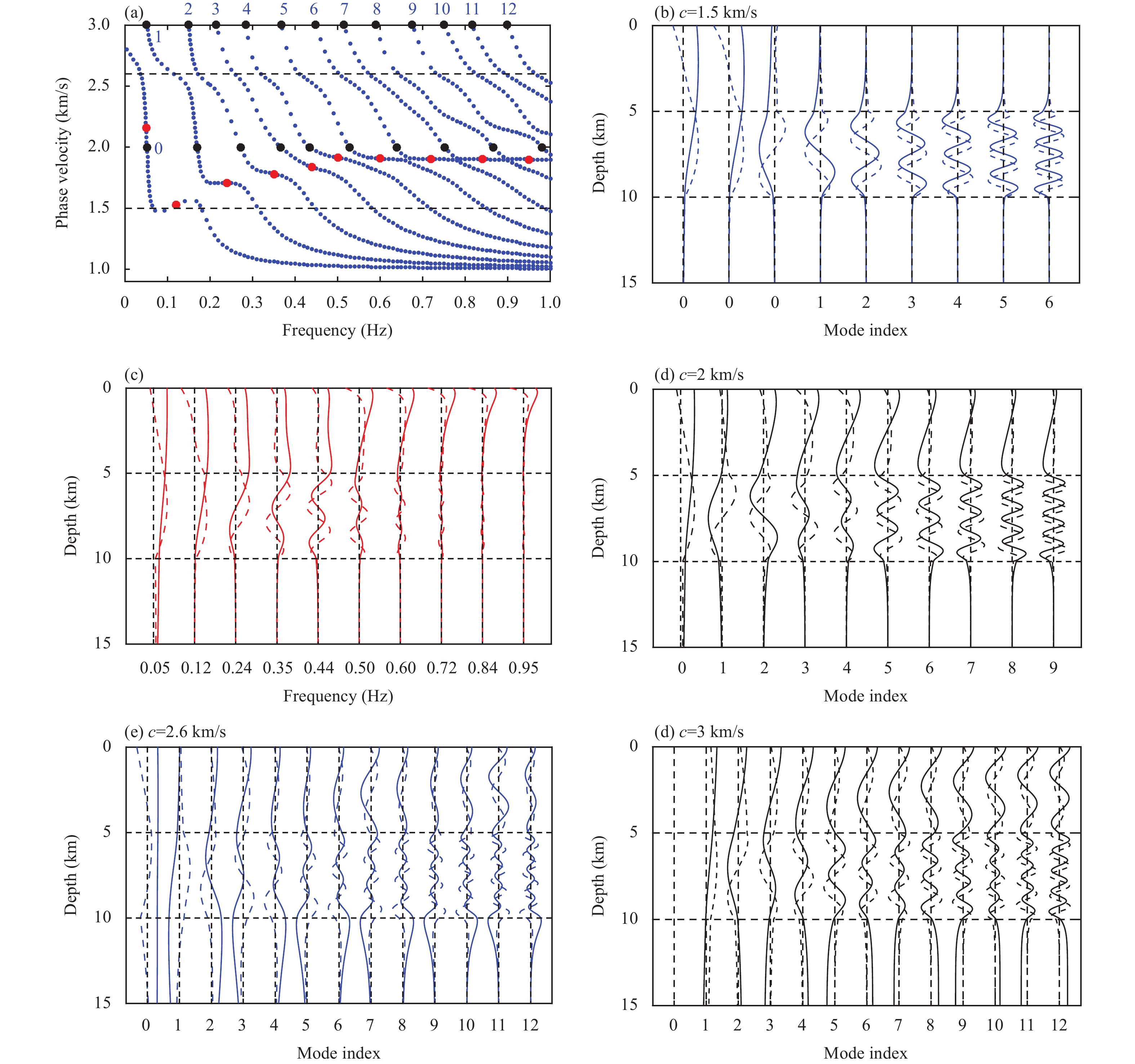
Figure 6 shows the eigenvalues and eigendisplacements of the P-SV system in Model 3. Figure 6b shows the eigendisplacement of the fundamental mode at f=0.6\;\mathrm{H}\mathrm{z} and c=0.943\;\mathrm{k}\mathrm{m}/\mathrm{s}. It decayed exponentially with depth and behaved as a typical characteristic of the fundamental Rayleigh wave mode. Figure 6c shows the eigendisplacement of the fundamental mode at critical phase velocity c=1.6\;\mathrm{k}\mathrm{m}/\mathrm{s}, similar to that in Figure 6b with a greater penetration depth. Figure 6d shows the eigendisplacements for the different modes at phase velocity c=1.6\;\mathrm{k}\mathrm{m}/\mathrm{s}. The energy was primarily concentrated in the first layer and decayed exponentially from z=5\;\mathrm{k}\mathrm{m}. The eigendisplacement characteristics shown in Figure 6d are typical for normal modes when the phase velocity is less than 2 km/s.
Figure
6.
Eigenvalues and eigendisplacement of P-SV wave in Model 3. (a) Phase velocity of Rayleigh waves. (b) Eigendisplacement associated with the eigenvalues denoted by a red dot in (a), where the frequency is 0.6 Hz and phase velocity is 0.943 km/s. (c) Eigendisplacement of the fundamental mode at 1 km/s. (d)–(j) denote the eigendisplacement at 1.6, 2, 2.2, 2.4, 2.5, 2.9, and 3 km/s, respectively. In the panels depicting eigendisplacement, blue denotes the normal mode, whereas black denotes the critical mode.
At c=2\;\mathrm{k}\mathrm{m}/\mathrm{s}, corresponding to the critical refraction of the SV wave in the first layer at z=5\;\mathrm{k}\mathrm{m}, the horizontal eigendisplacement in the second layer decayed exponentially, as shown in Figure 6c. For the vertical eigendisplacement, an additional linear term exists owing to the presence of an inhomogeneous P-wave. Consequently, it appears closer to a linear function than to an exponential one. Figure 6f and g shows the eigendisplacements at phase velocities c=2.2\;\mathrm{k}\mathrm{m}/\mathrm{s} and c=2.4\;\mathrm{k}\mathrm{m}/\mathrm{s}, respectively. They exhibited the typical characteristics of normal modes for 2\;\mathrm{k}\mathrm{m}/\mathrm{s} < c < 3\;\mathrm{k}\mathrm{m}/\mathrm{s}. The energy is primarily concentrated in the first and second layers and decays exponentially in the bottom half-space.
In contrast to the SH system, if the phase velocity is equal to the P-wave velocity of the first layer (2.5 km/s), the transfer matrix also exhibits a singularity. Figure 6h shows the eigendisplacement of the critical mode at c=2.5\;\mathrm{k}\mathrm{m}/\mathrm{s}. This was associated with the critical refraction of the P wave caused by the incident SV wave at z=5\;\mathrm{k}\mathrm{m} and the free surface at z=0\;\mathrm{k}\mathrm{m}. In the first layer, the horizontal eigendisplacement has a solution represented by triangular and linear functions. The solution for the vertical eigendisplacement follows a triangular function with a constant. Because of the weak effect of the linear function, the eigendisplacement characteristics shown in Figure 6h are similar to those shown in Figure 6f and g.
If the phase velocity was greater than 2.5\;\mathrm{k}\mathrm{m}/\mathrm{s}, a homogeneous P-wave was observed in the first layer. A homogeneous P-wave is observed in the region of the leaky mode in the dispersion branch, because the P-wave velocity in the layer is typically greater than the S-wave velocity in the bottom half-space. However, by setting a P-wave velocity smaller than the S-wave velocity in the half-space, a homogeneous P-wave can be observed in the region of the normal mode (De Nil, 2005). Two P-guided wave modes were observed from 2.5\;\mathrm{k}\mathrm{m}/\mathrm{s} < c < 3\;\mathrm{k}\mathrm{m}/\mathrm{s}. They appeared to intersect with the SV-guided waves. The eigendisplacements of the 7th mode at c=2.9\;\mathrm{k}\mathrm{m}/\mathrm{s}, as well as the 7th and 14th modes at c=3\;\mathrm{k}\mathrm{m}/\mathrm{s}, present typical characteristics of P-guided waves in the first layer, as shown in Figure 6i and j, respectively. The visual crossover between the dispersion branches of the P- and SV-guided waves may be due to the weak coupling between the P- and SV-waves. If the phase velocity was sufficiently high, the ray parameter approached zero. The rays were nearly vertically incident. The conversion coefficient between the P- and SV-waves tended to zero. The P- and SV-waves become nearly independent (Dahlen and Tromp, 1998). Consequently, two types of guided waves were generated: a P-guided wave with energy confined to the first layer, and an SV-guided wave with energy confined to the first and second layers. The Poisson’s ratio determines the relative velocities of the P and SV-wave, which in turn affects the separation of the P and SV waves. In general, the higher the Poisson’s ratio is, the larger the difference between the P- and S-wave velocities. P-guided waves are expected to be observed in the higher-phase velocity range and are more independent of SV-guided waves (Sun CY et al., 2021). All models in this study had relatively high Poisson’s ratios. The P-guided wave modes existed in all cases and appeared as leaky modes, except in Model 3. P-guided waves can be used to constrain the P-wave velocity structures during surface-wave inversion (Li J et al., 2018; Li ZB et al., 2021, 2022).
The critical mode at c=3\;\mathrm{k}\mathrm{m}/\mathrm{s} corresponds to the critical refraction of the SV-waves impinging on the interface of the lower half-space. As shown in Figure 6j, the horizontal eigendisplacement of the critical mode decays exponentially in the bottom half-space, whereas the vertical displacement remains constant with increasing depth because it has a solution with an exponential function plus a constant. Leaky modes can be observed if the phase velocity is higher than 3\;\mathrm{k}\mathrm{m}/\mathrm{s} (e.g., Shi CW et al., 2022). In this velocity range, a part of the energy of the SV-waves in the second layer leaks into the bottom half-space as a homogeneous plane wave. The roots of the dispersion equation are no longer real within the (+, +) Riemann sheet but are complex within the (+, –) Riemann sheet (Phinney, 1961).
4.3
Eigenvalues and eigendisplacement of the critical mode in the model with a low-velocity layer.
Figure 7 shows the eigenvalues and eigendisplacements of the SH wave in Model 4, in which a low-velocity layer is present. In contrast to Models 2 and 3, the high-frequency limit of the fundamental mode is no longer the S-wave velocity of the top layer but that of the low-velocity layer. Figure 7b shows the eigendisplacement of the modes at c=1.6\;\mathrm{k}\mathrm{m}/\mathrm{s}. This is a typical characteristic of the eigendisplacement for a phase velocity range of 1\;\mathrm{k}\mathrm{m}/\mathrm{s} < c < 2\;\mathrm{k}\mathrm{m}/\mathrm{s}. In addition to the lower mode at lower frequencies, the higher mode behaved as a guided wave whose energy was confined to a low velocity. As shown in Figure 7b, from the fundamental mode to the higher modes, the energy in the first layer gradually decreases and is concentrated in the lower velocity layer. Significant energy was observed only for the fundamental and first overtones in the first layer, primarily because of the tunneling effect at z=5\;\mathrm{k}\mathrm{m} in the low-frequency range. The energy in the first layer and bottom half-space gradually vanishes in higher modes. The energy concentration in the low-velocity layer is a typical guided or trapped wave. Therefore, if both the source and receiver are located at the surface, it is difficult to receive higher modes with velocities lower than 2 km/s, particularly in the mid- to high-frequency range. The received modes at the surface are primarily guided modes with velocities greater than or equal to 2 km/s, as illustrated by the eigendisplacements in Figure 7c–e. This is also illustrated by the numerical results (Luo YH et al., 2010).
Figure
7.
Eigenvalues and eigendisplacement of SH wave in Model 3. (a) Phase velocity of a Love wave. (b) and (c) are the eigendisplacement of modes at phase velocities of 1.6 and 2 km/s, respectively. (d) Eigendisplacement associated with the eigenvalues denoted by green dots in (a). (e) and (f) are the eigendisplacement of modes at phase velocities of 2.6 and 3 km/s, respectively.
Figure 7c shows the eigendisplacement of the critical mode at c=2\;\mathrm{k}\mathrm{m}/\mathrm{s}. Compared to the typical normal mode, the distinctive feature of the critical mode is that evident energy can be observed in the top layer, and the eigendisplacement of the critical mode remains constant in this layer. This implies that, at the critical refraction, the guided waves in the low-velocity layer also radiate energy to the top layer. The eigendisplacement remains a frequency-independent constant in the top layer and rapidly decays to zero in the bottom half-space. The top layer behaves like an open half-space upward, which is the reason we exchanged the definition of the up- and down-going waves of the first layer in Equation (26), as described in Section 3.2.2. If the phase velocity is greater than c=2\;\mathrm{k}\mathrm{m}/\mathrm{s} and less than c=3\;\mathrm{k}\mathrm{m}/\mathrm{s}, the eigendisplacement in the first layer, which behaves as a constant at c=2\;\mathrm{k}\mathrm{m}/\mathrm{s} , gradually transitions into a triangular function, as shown in Figure 7e, where the eigendisplacement at c=2.6\;\mathrm{k}\mathrm{m}/\mathrm{s} is given. The eigendisplacement shown in Figure 7e was concentrated in the first and second layers and decayed exponentially in the bottom half-space, exhibiting typical characteristics of the normal mode.
Figure 7f shows the eigendisplacement of the critical mode, where the phase velocity is equal to the S-wave velocity in the bottom half-space (3 km/s). The characteristics of the first and second layers were similar to those shown in Figure 7e. The main difference is that the energy of the critical mode does not decay with depth and remains constant in the bottom half-space.
Near the critical mode at c=2\;\mathrm{k}\mathrm{m}/\mathrm{s}, at frequencies higher than 0.3 Hz, a segment exists along the dispersion branches where the gradient change of phase velocity is small, as shown by the green dots in Figure 7a. These eigenvalues represent the SV-guided waves that undergo back-and-forth reflections in the first layer. Figure 7d shows the eigendisplacements associated with the eigenvalues denoted by the green dots in Figure 7a . Although these eigenvalues are close to those of the critical mode, the eigendisplacements of these modes do not remain constant in the first layer. Compared to the normal modes shown in Figure 7e, the eigendisplacements in Figure 7d exhibited a frequency-independent feature in the first layer. This is due to the solotone effect in the first layer (Kennett and Kerry, 1979; Lapwood and Usami, 1981). These SH-guided waves can be understood as the constructive interference of the SH plane waves in the first layer, which leak energy into the second layer as leaky modes.
Figure 8 shows the eigenvalues and eigendisplacements of the P-SV system in Model 4. The characteristics of the Rayleigh wave dispersion curve for a model with a low-velocity layer are of concern to many researchers because they are often encountered in practice.
Figure
8.
Eigenvalues and eigendisplacement of P-SV wave in Model 4. (a) Phase velocity of a Rayleigh wave. (b) Eigendisplacement at the phase velocity of 1.5 km/s. (c) Eigendisplacement associated with the eigenvalues denoted by red dots in (a). (d)–(f) are eigendisplacements at phase velocities of 2, 2.6, 3 km/s, respectively.
Figure 8a shows the dispersion curves of the Rayleigh wave mode. Mode kissing can be observed if the frequency exceeds a given value, such as 0.6 Hz for Model 4. Zhang BX and Lu LY (2002) studied this phenomenon based on the energy distribution in each mode. Liu XF et al. (2009) investigated this phenomenon via numerical simulations. This is likely due to the interaction between the two waves propagating independently. These are the SV-guided waves within the low-velocity layer and free-surface Rayleigh waves. At frequencies greater than 0.6 Hz, the phase velocities of the free-surface Rayleigh wave are similar to those of the classic Rayleigh wave propagating in the supposed half-space formed by the top layer. These phase velocities are visually a straight line connected by the red dots shown in Figure 8a, because the classic Rayleigh wave in half-space is independent of frequency. The dispersion branches of the SV-guided wave pass through this straight line.
At frequencies less than 0.6 Hz, the modes with maximum energy at the surface are indicated by red dots. Figure 8c shows the eigendisplacements corresponding to the eigenvalues denoted by the red dots in Figure 8a. At frequencies less than 0.6 Hz, a significant energy distribution can be observed in the top layer and the low-velocity layer, exhibiting characteristics of free surface Rayleigh and SV-guided waves. This implies that the inhomogeneous P- and SV-waves emitted from the surface radiate into the low-velocity layer. As the frequency increases, the energy concentrates towards the surface. Starting from the 5th mode (approximately 0.6 Hz), the eigendisplacements behave as free-surface Rayleigh waves, and the phase velocities of the modes with maximum energy are distributed along the visually straight line.
In seismic exploration, the measured dispersion curve extracted from the data at the surface is formed by the curve that connects the red dots in Figure 8a, and “jumps” between different modes. The measured mode is referred to as the “effective mode” (Foti, 2000) or the “R mode” (FanYH et al., 2007). Wu B (2016) referred to this mode as the physically meaningful “fundamental” mode. This is an extension of the classical Rayleigh-wave mode. In contrast, the fundamental mode (labeled 0 in Figure 8a), which is formed by the lowest velocities for a given frequency, does not behave as an extension of the classic Rayleigh wave mode at high frequencies.
Figure 8b shows the eigendisplacements of the critical mode at c=1.5\;\mathrm{k}\mathrm{m}/\mathrm{s}, that is, the eigendisplacement associated with the eigenvalues given by the intersections between the black dashed line (representing c=1.5\;\mathrm{k}\mathrm{m}/\mathrm{s}) and the dispersion branches in Figure 8a. The first two eigendisplacements, labeled as the 0th mode, are associated with the eigenvalues of the fundamental mode around the red dots in Figure 8a. They exhibit the characteristics of a free-surface Rayleigh wave, with the energy primarily concentrated in the first and second layers, particularly near the surface. The energies of the other modes, labeled 1 to 6, were primarily concentrated within the low-velocity layer.
Figure 8d shows the eigendisplacements of the critical mode at c=2\;\mathrm{k}\mathrm{m}/\mathrm{s}. In contrast to the SH system shown in Figure 7c, energy can be observed in both the first and second layers of the P-SV system rather than being confined within the low-velocity layer. This can be attributed to inhomogeneous P-waves, which allow for a nonzero solution with a linear function of the SV wave in the first layer. Consequently, the vertical eigendisplacement in the first layer exhibits a shape that is closer to a linear function. However, in the bottom half-space, the eigendisplacement rapidly decreased to zero.
When the phase velocity is greater than 2\;\mathrm{k}\mathrm{m}/\mathrm{s}, the distribution of the eigendisplacement in the first layer gradually changes from nearly linear to nearly sinusoidal, as shown in Figure 8e, where the eigendisplacement at c=2.6\;\mathrm{k}\mathrm{m}/\mathrm{s} is given. In addition, the attenuation in the bottom half-space becomes slow, and significant energy is observed in the bottom half-space for the lower modes.
Figure 8f shows the eigendisplacement of the critical mode at c=3\;\mathrm{k}\mathrm{m}/\mathrm{s}. Their distributions in the first and second layers were similar to those at c=2.6\;\mathrm{k}\mathrm{m}/\mathrm{s}, as shown in Figure 8e. The main difference is that, for the critical mode, the eigendisplacement in the bottom half-space remains constant and does not decay with depth.
5.
On the zero frequency
In addition to the critical mode, where the phase velocity is equal to the velocity of the body waves of the layer, there is a special zero-frequency point.
At the zero-frequency, the solution of Equation (23) in the time domain is similar to that of Equation (26), which can be expressed as a linear function of time, that is, {T}\left(t\right)={C}_{1}+{C}_{2}t. Considering that displacement cannot increase indefinitely with time, {C}_{2}t vanishes. Then, the solution of Equation (23) is a static displacement. The calculation of the static displacement field at zero frequency can be found in the study by Xie XB and Yao ZX (1989). When calculating the eigenvalues and eigenfunctions, defining the phase velocity of a static field at zero frequency is challenging. An alternative is to analyze the limits of the phase velocity and eigenfunction as the frequency approaches zero.
When the frequency approaches zero, the exponential decay in the half-space is extremely slow and the penetration depth is large. The horizontal layered model is governed mainly by the behavior of the bottom half-space and degenerates into a homogeneous half-space model. As analyzed in Section 4.2, for the Love wave, the zero-frequency limit is the S-wave velocity of the bottom half-space, and for the Rayleigh wave, it is the classic Rayleigh wave phase velocity of the bottom half-space. This demonstrates the importance of calculating the critical modes, particularly the critical mode of the SH wave in the homogeneous half-space, which provides a theoretical basis for estimating the limit of Love waves in a layered medium when the frequency tends to zero. As discussed in Section 4.1, in a homogeneous half-space, a critical mode exists with a phase velocity equal to the S-wave velocity.
When the frequency approaches zero, considering the solutions of the eigendisplacement in Equation (27) for each layer, whether it is a homogeneous (trigonometric function) or an inhomogeneous (exponential function) plane wave, the eigendisplacement tends to be constant, as demonstrated by the fundamental-mode eigendisplacement shown in Figure 3c.
6.
Discussion and conclusions
In this study, the eigenvalues and eigenfunctions of the critical modes, where the phase velocity is equal to the body wave velocity in the layer, were investigated based on the theoretical framework of the GRT. By embedding the linear solution of the wave equation at zero vertical wavenumber into the framework of the GRT theory, the singularity of the critical modes is addressed. The singularity arises in the original GRT theory matrix formulation when the phase velocity is the same as the body-wave velocity of each layer and the general solution of the wave equation at zero vertical wavenumbers is not considered. This singularity makes the secular function close to zero near the critical phase velocity at any given frequency. Wu B and Chen XF (2016) exclude the roots that cause the secular function to vanish as branch points without further explanation. The secular function is zero for the critical mode because the solution is obtained by modifying the matrix formulation and considering the linear solution of the wave equation at the critical phase velocity. These critical modes correspond to critical reflection, transmission, and grazing incidence phenomena, which are closely related to head waves (Červený, 1971), apparent head waves (Zhang J et al., 2002), and downward head waves (Wang BW and Zhao HR, 1986). The characteristics of the critical mode eigenfunctions were studied for homogeneous half-space and layered models. In contrast to the normal mode in which the eigenfunctions decay exponentially in the bottom half-space of the horizontally multilayered model, the eigenfunctions are constant in the bottom half-space and do not decay with depth for the critical mode whose phase velocity equal to S velocity in the bottom half-space. This is because the horizontally layered model is an open system with the bottom half-space tending to infinity.
Bounded by the phase velocity of the critical mode, that is, the body wave velocity of each layer, the dispersion curves can be divided into different regions. The characteristics of the eigenvalues and eigenfunctions for the different velocity regions were investigated. The different characteristics of the different velocity regions are related to the reflection and transmission paths caused by body waves incident at different angles within the layers. Different phase velocity regions reflect different ray distributions and different phase velocity regions exhibit different P- and S-wave behaviors, such as propagation, evanescence, and trapped characteristics (Kennett, 2023). Rays can be classified according to their incidence angle (e.g., incidence less than the critical angle, critical incidence, and supercritical incidence). Subsequently, the relationship between the ray paths and modes within different velocity ranges should be investigated. These issues will be addressed in a separate study.
Although seismic wave propagation in horizontally layered media is a classical problem, analyzing the characteristics of normal and leaky modes in such simple models is still of theoretical and practical significance.
First, traditional surface-wave inversion is based on dispersion curves, which require the identification of the mode branches. Theoretical dispersion curves of the predicted model were fitted to the observed values. However, two potential risks arise during this process. One is mode misidentification (Gao LL et al., 2014, 2016), and the other is missing modes in the calculations for theoretical dispersion (Shi CW et al., 2022). Mode misidentification is particularly evident when “mode kissing” occurs between two branches. The missing mode was related to the numerical treatment used to calculate the theoretical dispersion curves. Both the mode misidentification of the measured dispersion curves and the missing mode of the predicted dispersion curves would theoretically introduce significant errors into the inversion. The inversion method, which compares the theoretical and observed spectra in the frequency-velocity domain, is an alternative to surface wave inversion that does not require knowledge of the dispersion curves. However, it is essential to know the mode interaction, characteristics of the eigenvalues and eigenfunctions of modes (normal modes and leaky modes), and their spectral characteristics in the frequency-velocity domain (Kennett et al., 2023). The inversion of the spectra-based method avoids the issues associated with inversion based on dispersion curves.
Second, with the development of a three-dimensional array, it is possible to directly measure the energy distribution of the modes along depth (Meyers et al., 2019). Studying the distribution of eigenfunctions at different depths aids our understanding of the relationship between modes and ray paths and the sensitivity of modes to depth-dependent parameters. This lays the foundation for directly inferring medium parameters based on mode eigenfunctions (Glubokovskikh et al., 2021; Huff et al., 2021).
Acknowledgment
This study was supported by the National Natural Science Foundation of China (No. U1839209). We would like to thank the associate editor and two anonymous reviewers for their valuable suggestions and comments, which helped us refine the manuscript.
Conflict of interest
The authors affirm that they have no financial and personal relationships with any individuals or organization that could have potentially influenced the work presented in this paper.
Chimenti DE, Nayfeh AH and Butler DL (1982). Leaky Rayleigh waves on a layered halfspace. J Appl Phys 53(1): 170–176 https://doi.org/10.1063/1.329913.
Červený V, and Ravindra R (1971). Theory of Seismic Head Waves. University of Toronto Press, Toronto.
Dahlen FA, and Tromp J (1998). Theoretical Global Seismology. Princeton University Press, Princeton.
De Nil D (2005). Characteristics of surface waves in media with significant vertical variations in elasto-dynamic properties. Environ Eng Geophys 10(3): 263–274 https://doi.org/10.2113/jeeg10.3.263.
Dunkin JW (1965). Computation of modal solutions in layered, elastic media at high frequencies. Bull Seismol Soc Am 55(2): 335–358 https://doi.org/10.1785/bssa0550020335.
Ewing WM, Jardetzky WS and Press F (1957). Elastic Waves in Layered Media. McGraw-Hill Book Company, New York.
Fan YH, Chen XF, Liu XF, Liu JQ and Chen XH (2007). Approximate decomposition of the dispersion equation at high frequencies and the number of multimodes for Rayleigh waves. Chin J Geophys 50(1): 233–239 https://doi.org/10.3321/j.issn:0001-5733.2007.01.029 (in Chinese with English abstract).
Foti S (2000). Multistation methods for geotechnical characterization using surface waves. Dissertation. Poletechnic di Torino, Torino.
Fu L, Pan L, Li ZB, Dong S, Ma QB and Chen XF (2022). Improved high-resolution 3D vS model of long beach, CA: inversion of multimodal dispersion curves from ambient noise of a dense array. Geophys Res Lett 49(4): e2021GL097619 https://doi.org/10.1029/2021gl097619.
Gao LL, Xia JH and Pan YD (2014). Misidentification caused by leaky surface wave in high-frequency surface wave method. Geophys J Int 199(3): 1452 – 1462 https://doi.org/10.1093/gji/ggu337.
Gao LL, Xia JH, Pan YD and Xu YX (2016). Reason and condition for mode kissing in MASW method. Pure Appl Geophys 173(5): 1627 – 1638 https://doi.org/10.1007/s00024-015-1208-5.
Gilbert F and Backus GE (1966). Propagator matrices in elastic wave and vibration problems. Geophysics 31(2): 326 – 332 https://doi.org/10.1190/1.1439771.
Glubokovskikh S, Pevzner R, Sidenko E, Tertyshnikov K, Gurevich B, Shatalin S, Slunyaev A and Pelinovsky E (2021). Downhole distributed acoustic sensing provides insights into the structure of short-period ocean-generated seismic wavefield. J Geophys Res:Solid Earth 126(12): e2020JB021463 https://doi.org/10.1029/2020jb021463.
Haddon RAW (1984). Computation of synthetic seismograms in layered earth models using leaking modes. Bull Seismol Soc Am 74(4): 1225 – 1248 https://doi.org/10.1785/bssa0740041225.
Haddon RAW (1986). Exact evaluation of the response of a layered elastic medium to an explosive point source using leaking modes. Bull Seismol Soc Am 76(6): 1755 – 1775 https://doi.org/10.1785/bssa0760061755.
Harkrider DG (1964). Surface waves in multilayered elastic media I. Rayleigh and Love waves from buried sources in a multilayered elastic half-space. Bull Seismol Soc Am 54(2): 627 – 679 https://doi.org/10.1785/bssa0540020627.
He YF, Chen WT and Chen XF (2006). Normal mode computation by the generalized reflection_transmission coefficient method in planar layered half space. Chin J Geophys 49(4): 1074 – 1081 https://doi.org/10.3321/j.issn:0001-5733.2006.04.020 (in Chinese with English abstract).
Hu SQ, Luo S and Yao HJ (2020). The frequency-Bessel spectrograms of multicomponent cross-correlation functions from seismic ambient noise. J Geophys Res:Solid Earth 125(8): e2020JB019630 https://doi.org/10.1029/2020jb019630.
Huff O, Luo B, Lellouch A and Jin G (2021). An eigenfunction representation of deep waveguides with application to unconventional reservoirs. Geophysics 86(6): T509 – T521 https://doi.org/10.1190/geo2021-0201.1.
Lapwood ER and Usami T (1981). Free Oscillations of the Earth. Cambridge University Press, Cambridge.
Li J, Hanafy S and Schuster G (2018). Wave-equation dispersion inversion of guided P waves in a waveguide of arbitrary geometry. J Geophys Res:Solid Earth 123(9): 7760 – 7774 https://doi.org/10.1029/2018jb016127.
Li ZB, Shi CW and Chen XF (2021). Constraints on crustal P wave structure with leaking mode dispersion curves. Geophys Res Lett 48(20): e2020GL091782 https://doi.org/10.1029/2020gl091782.
Li ZB, Shi CW, Ren HX and Chen XF (2022). Multiple leaking mode dispersion observations and applications from ambient noise cross-correlation in Oklahoma. Geophys Res Lett 49(1): e2021GL096032 https://doi.org/10.1029/2021gl096032.
Liu XF, Fan YH and Chen XF (2009). Research on the cross of the dispersion curves of Rayleigh waves and multi-modes coupling phenomenon. Chin J Geophys 52(9): 2302 – 2309 https://doi.org/10.3969/j.issn.0001-5733.2009.09.014 (in Chinese with English abstract).
Luco JE and Apsel RJ (1983). On the Green’s functions for a layered half-space. Part I. Bull Seismol Soc Am 73(4): 909 – 929 https://doi.org/10.1785/bssa0730040909.
Luo YH, Xia JH, Xu YX, Zeng C and Liu JP (2010). Finite-difference modeling and dispersion analysis of high-frequency Love waves for near-surface applications. Pure Appl Geophys 167(12): 1525 – 1536 https://doi.org/10.1007/s00024-010-0144-7.
Maupin V (1996). The radiation modes of a vertically varying half-space: a new representation of the complete Green’s function in terms of modes. Geophys J Int 126(3): 762 – 780 https://doi.org/10.1111/j.1365-246x.1996.tb04701.x.
Mellman GR and Helmberger DV (1974). High-frequency attenuation by a thin high-velocity layer. Bull Seismol Soc Am 64(5): 1383 – 1388 https://doi.org/10.1785/bssa0640051383.
Meyers P, Bowden DC, Prestegard T, Tsai VC, Mandic V, Pavlis G and Caton R (2019). Direct observations of surface-wave eigenfunctions at the homestake 3D array. Bull Seismol Soc Am 109(4): 1194 – 1202 https://doi.org/10.1785/0120190026.
Pei D, Louie JN and Pullammanappallil SK (2008). Improvements on computation of phase velocities of Rayleigh waves based on the generalized R/T coefficient method. Bull Seismol Soc Am 98(1): 280 – 287 https://doi.org/10.1785/0120070057.
Phinney RA (1961). Leaking modes in the crustal waveguide: 1. The oceanic PL wave. J Geophys Res 66(5): 1445 – 1469 https://doi.org/10.1029/jz066i005p01445.
Qin TW, Lu LY, Ding ZF, Feng XZ and Zhang YY (2022). High-resolution 3D shallow S wave velocity structure of Tongzhou, subcenter of Beijing, inferred from multimode Rayleigh waves by beamforming seismic noise at a dense array. J Geophys Res:Solid Earth 127(5): e2021JB023689 https://doi.org/10.1029/2021jb023689.
Qin TW and Lu LY (2022). A Modified Cross-correlation Beamforming (MCBF) for extracting multimode surface wave dispersion curves from ambient seismic noise. ESS Open Archive. https://doi.org/10.1002/essoar.10511872.1.
Saito M (1967). Excitation of free oscillations and surface waves by a point source in a vertically heterogeneous earth. J Geophys Res 72(14): 3689 – 3699 https://doi.org/10.1029/jz072i014p03689.
Shi CW, Ren HX, Li ZB and Chen XF (2022). Calculation of normal and leaky modes for horizontal stratified models based on a semi-analytical spectral element method. Geophys J Int 230(3): 1928 – 1947 https://doi.org/10.1093/gji/ggac163.
Sun CY, Wang ZN, Wu DS, Cai RQ and Wu H (2021). A unified description of surface waves and guided waves with relative amplitude dispersion maps. Geophys J Int 227(3): 1480 – 1495 https://doi.org/10.1093/gji/ggab284.
Thomson WT (1950). Transmission of elastic waves through a stratified solid medium. J Appl Phys 21(2): 89 – 93 https://doi.org/10.1063/1.1699629.
Wu B and Chen XF (2016). Stable, accurate and efficient computation of normal modes for horizontal stratified models. Geophys J Int 206(2): 1281 – 1300 https://doi.org/10.1093/gji/ggw209.
Wu B (2016). The theory of normal modes of surface waves and Earth′s free oscillations. Dissertation. University of Science and Technology of China, Hefei (in Chinese with English abstract).
Xia JH, Miller RD, Park CB and Tian G (2003). Inversion of high frequency surface waves with fundamental and higher modes. J Appl Geophys 52(1): 45 – 57 https://doi.org/10.1016/s0926-9851(02)00239-2.
Xie XB and Yao ZX (1989). A generalized reflection-transmition coefficient matrix method to calculate static displacement field of a stratified half-space by dislocation source. Acta Geophys Sin 32(3): 270– 280 (in Chinese with English abstract).
Yang HY, Zhao L and Hung SH (2010). Synthetic seismograms by normal-mode summation: a new derivation and numerical examples. Geophys J Int 183(3): 1613 – 1632 https://doi.org/10.1111/j.1365-246x.2010.04820.x.
Zhang BX, Yu M, Lan CQ and Xiong W (1996). Elastic wave and excitation mechanism of surface waves in multilayered media. J Acoust Soc Am 100(6): 3527 – 3538 https://doi.org/10.1121/1.417329.
Zhang HM (2021). Lamb Problem in Seismology. Science Press, Beijing.
Zhang J, Zhang HM and Chen XF (2002). Characteristics of head wave in multi-layered half space. Acta Seismol Sin 24(6): 559 – 568 https://doi.org/10.3321/j.issn:0253-3782.2002.06.001 (in Chinese with English abstract).

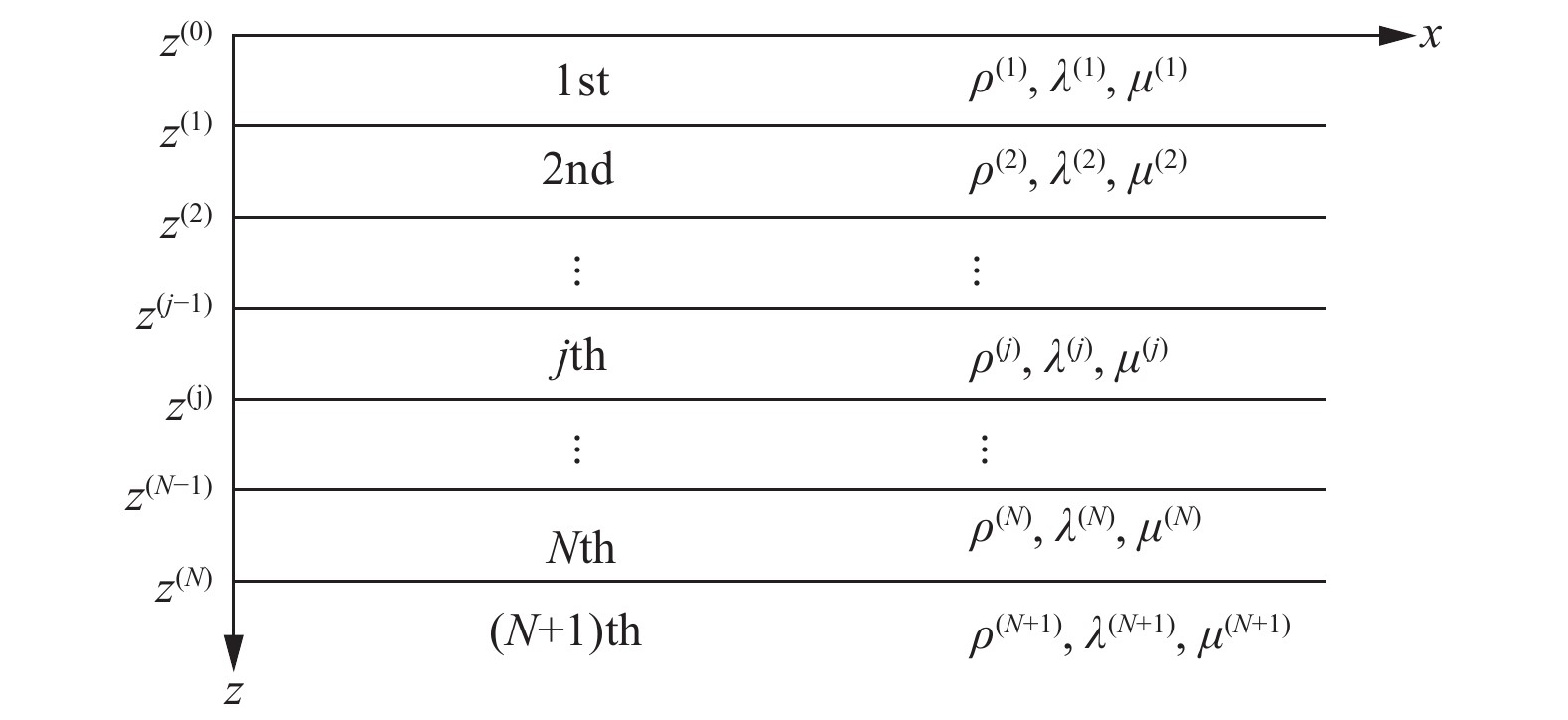
 DownLoad: