Liu YJ, Zhao XF, Wen ZP, Liu J, Chen B, Bu CY and Xu C (2023). Broadband ground motion simulation using a hybrid approach of the May 21, 2021 M7.4 earthquake in Maduo, Qinghai, China. Earthq Sci 36(3): 175–199,. DOI: 10.1016/j.eqs.2023.04.001
Citation:
Liu YJ, Zhao XF, Wen ZP, Liu J, Chen B, Bu CY and Xu C (2023). Broadband ground motion simulation using a hybrid approach of the May 21, 2021 M7.4 earthquake in Maduo, Qinghai, China. Earthq Sci 36(3): 175–199,. DOI: 10.1016/j.eqs.2023.04.001
Liu YJ, Zhao XF, Wen ZP, Liu J, Chen B, Bu CY and Xu C (2023). Broadband ground motion simulation using a hybrid approach of the May 21, 2021 M7.4 earthquake in Maduo, Qinghai, China. Earthq Sci 36(3): 175–199,. DOI: 10.1016/j.eqs.2023.04.001
Citation:
Liu YJ, Zhao XF, Wen ZP, Liu J, Chen B, Bu CY and Xu C (2023). Broadband ground motion simulation using a hybrid approach of the May 21, 2021 M7.4 earthquake in Maduo, Qinghai, China. Earthq Sci 36(3): 175–199,. DOI: 10.1016/j.eqs.2023.04.001
• The validation results demonstrate the ability of the hybrid simulation methodology to reproduce the main characteristics of the observed ground motions for the 2021 Maduo earthquake.
• The map of macroseismic intensity tends overestimate the shaking intensity by one intensity unit.
• Comparisons indicate a general good consistency between the simulated and empirical predicted intensity measures only for the short period.
• The low frequency components of ground motions of the Maduo earthquake were not prominent.
Abstract
In this study, the broadband ground motions of the 2021 M7.4 Maduo earthquake were simulated to overcome the scarcity of ground motion recordings and the low resolution of macroseismic intensity map in sparsely populated high-altitude regions. The simulation was conducted with a hybrid methodology, combining a stochastic high-frequency simulation with a low-frequency ground motion simulation, from the regional 1-D velocity structure model and the Wang WM et al. (2022) source rupture model, respectively. We found that the three-component waveforms simulated for specific stations matched the waveforms recorded at those stations, in terms of amplitude, duration, and frequency content. The validation results demonstrate the ability of the hybrid simulation method to reproduce the main characteristics of the observed ground motions for the 2021 Maduo earthquake over a broad frequency range. Our simulations suggest that the official map of macroseismic intensity tends to overestimate shaking by one intensity unit. Comparisons of simulations with empirical ground motion models indicate generally good consistency between the simulated and empirically predicted intensity measures. The high-frequency components of ground motions were found to be more prominent, while the low-frequency components were not, which is unexpected for large earthquakes. Our simulations provide valuable insight into the effects of source complexity on the level and variability of the resulting ground motions. The acceleration and velocity time histories and corresponding response spectra were provided for selected representative sites where no records were available. The simulated results have important implications for evaluating the performance of engineering structures in the epicentral regions of this earthquake and for estimating seismic hazards in the Tibetan regions where no strong ground motion records are available for large earthquakes.
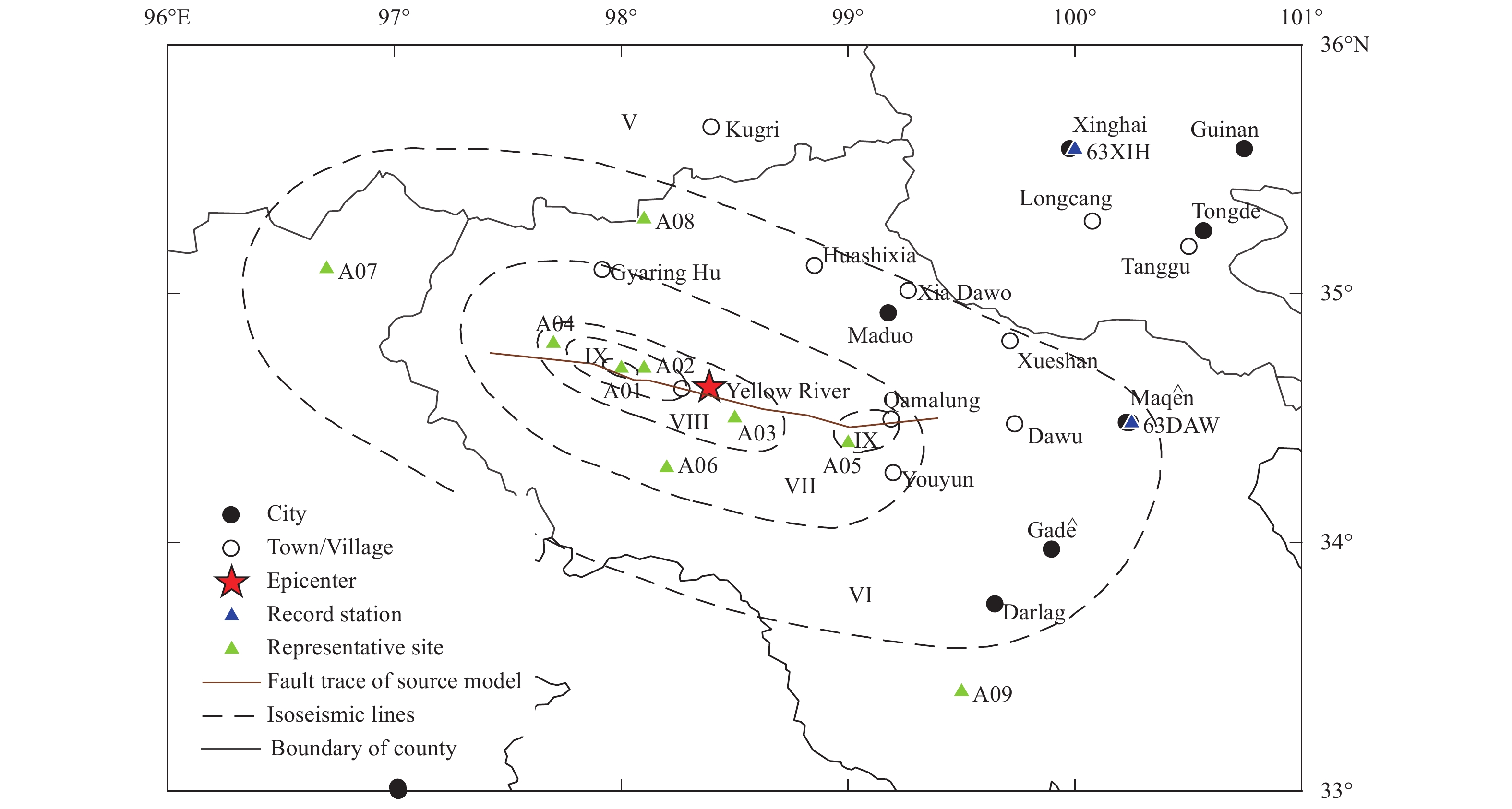
On May 21, 2021, an M7.4 earthquake occurred in Maduo, Qinghai province, Northwest China, located on the top of the Tibetan Plateau (hereinafter referred to as the Maduo earthquake). The epicenter, as determined by the China Earthquake Network Center, was located at 34.59°N and 98.34°E. Figure 1 shows a surface projection map of the study area associated with the event. Notably, the Maduo earthquake caused much destruction in the high-altitude inland eastern Tibetan Plateau, resulting in many casualties and severe damage. In particular, in the epicentral region, infrastructure such as roads and bridges suffered considerable damage, and some bridges even collapsed (such as the Changmahe Bridge on provincial highway S219). Additionally, soil liquefaction occurred in the near-fault region.
The Maduo earthquake has generated widespread interest among the Chinese scientific community. The China Earthquake Administration released a shakemap of macroseismic intensity distribution for the Maduo earthquake. Ren JJ et al. (2022) conducted field observations and detailed measurements for the Maduo coseismic surface rupture and measured 114 offsets in situ. Their results indicate prominent surface breaks characterized by discontinuous shear faults, a dominantly left-lateral strike-slip motion with a maximum sinistral offset of ~2.7–2.8 m, and general offset of ~1.0–1.5 m. The west part of the Maduo surface rupture zone occurred along the Jiangcuo fault, and its east portion cut through some west-northwest-trending tectonics. To examine the source rupture characteristics of the Maduo earthquake, Wang WM et al. (2022) combined thirty far-field P waves, twenty-six SH waveforms, and INSAR coseismic displacement data into a joint inversion to construct the finite source fault model for the Maduo earthquake. Using seismic and geodetic data, Zhang X et al. (2022) investigated the spatiotemporal rupture complexity of the Maduo earthquake, and categorized it as a supershear event, with rupture propagating bilaterally towards both the west and the east. Using geodetic and seismic observations, Chen KJ et al. (2022) modeled the temporal evolution of fault slip during the earthquake, revealing that a slip-pulse ruptured 170 km along the fault system with a horizontal shear slip of up to 4.2 m. Liu CY et al. (2021) combined interferometric synthetic aperture radar, GPS, and teleseismic data to study the coseismic slip distribution, fault geometry, and dynamic source rupture process of the Maduo earthquake. Li Q et al.′s (2022) results indicate that the earthquake was a bilateral rupture event with asymmetric rupture velocities; the rupture velocity in the east was higher than that in the west and may have reached supershear velocity. Using 1-Hz GNSS displacement waveforms, GNSS static offsets, and SAR observations, Lyu MZ et al. (2022) indicated that this event spread bilaterally with asymmetric rupture velocities of 3.8 km/s to the southeast of the epicenter and 2.2 km/s to the northwest. Yue H et al. (2022) conducted a joint inversion for this earthquake and resolved a bilateral rupture process characterized by both super- and sub-shear rupture velocities.
However, some important issues still need to be addressed. The shakemap of the macroseismic intensity distribution for the Maduo earthquake has a very low resolution, with large uncertainty in the sparsely populated and high-altitude regions. This is because the epicentral region contains few buildings from which to infer macroseismic intensity. Therefore, alternative methods are needed, such as the strong ground motion method, to determine a more detailed shakemap of macroseismic intensity distribution. However, observing strong ground motion is made difficult by the infrequency of large earthquakes (Lee et al., 2003), especially in sparsely populated high-altitude regions. The Maduo earthquake occurred in the Bayan Har block along the eastern margin of the Tibetan Plateau, a sparsely populated area with a general elevation of 4100–4200 m. Unfortunately, the epicentral region of this event did not contain any strong ground motion stations, and no near-field strong ground motions were recorded for this large earthquake. This event only triggered 16 strong motion stations within the National Strong Motion Observation Network System (NSMONS) of China. Strong ground motions with a maximum peak ground acceleration (PGA) of 45.95 cm/s2 were recorded at station 63DAW, 175.47 km from the epicenter. However, most of these far-field recordings have no engineering significance. This lack of strong ground motion recordings has hindered direct estimations of ground shaking intensity, duration, and frequency which are required to understand earthquake behavior and to evaluate the performance of engineered structures during an earthquake. Therefore, simulated ground motions during the Maduo earthquake are required to conduct such estimations.
Deterministic physics-based, stochastic, or hybrid models can be used to numerically simulate ground motions. Physics-based models are attractive because they alleviate the need to explicitly prescribe the kinematic rupture process, which, in many instances, must be based on simplified assumptions and approximations (Graves and Pitarka, 2004, 2010). Unfortunately, the current realization of earthquake rupture dynamics is limited and suffers from a scarcity of direct observations and measurements, especially for those processes affecting the propagation of high-frequency ground motions (Graves and Pitarka, 2010). In contrast, stochastic models are generally simpler to generate and consequently are more convenient to use than deterministic physics-based models (Beresnev and Atkinson, 1997; Boore, 2003). Additionally, in many cases, these models are more accurate in simulating high-frequency ground motions. Alternatively, hybrid models can compute low- and high-frequency ground motions separately and then combine them to produce a single time series of shaking (Hartzell et al., 1999).
The hybrid broadband ground motion simulation method developed by Graves and Pitarka (2010) (hereafter referred to as the GP method) may provide useful insights into strong ground motions resulting from the 2021 M7.4 Maduo earthquake at regional and specific sites, to overcome the limitation of strong motion scarcity. The GP method has been used to successfully simulate broadband ground motions during the 1933 Long Beach earthquake (Hough and Graves, 2020), the 1906 San Francisco earthquake (Aagaard et al., 2008), the 1989 Loma Prieta earthquake (Graves and Pitarka, 2010), the 2011 Christchurch earthquake (Razafindrakoto et al., 2018), the 2019 Ridgecrest earthquake (Pitarka et al., 2021), and in other scenarios (Graves et al., 2008). In this study, synthetic broadband strong ground motions were simulated using the GP method. We used this method to simulate ground motions at specific sites and compute the spatial distribution of ground motion intensity measurements (PGA, peak ground acceleration; PGV, peak ground velocity; and SAs, acceleration response spectra) in the region where strong earthquake ground motion recordings were not available. These broadband simulations of strong ground motions have important applications in further analysis of earthquake damage to engineering structures near faults and for evaluating the performance of engineering structures. In addition, this study provides a basis for the future implementation of probabilistic seismic hazard analysis (PSHA) and seismic design on the Tibetan Plateau.
The hybrid broadband ground motion simulation methodology of Graves and Pitarka (2004, 2010) was used to compute ground motions for the 2021 M7.4 Maduo earthquake. This method combines a deterministic finite-difference calculation for frequencies f < 1.0 Hz with a stochastic calculation for frequencies 1.0 Hz < f < 20.0 Hz. The stochastic approach follows a semi-empirical ray-based theory that contains a stochastic source radiation pattern and simplified wave propagation through a 1D-layered approximate velocity model.
2.1.1
Low-frequency simulation (f < 1 Hz)
The low-frequency simulation methodology uses a theoretical rigorous representation of the source and wave propagation effects, derived from the elastic dynamics equation. It incorporates both complex source rupture and wave propagation effects within an arbitrarily heterogeneous three-dimensional (3D) geologic structure. The basic calculation was carried out using a (3D) viscoelastic finite-difference algorithm (Graves, 1996; Day and Bradley, 2001), which was solved by implementing a staggered-grid finite-difference method to obtain fourth-order spatial and second-order temporal accuracies. Applications of this finite-difference methodology have been described by Graves (1996) and Pitarka (1999).
The moment tensor components are represented as an equivalent distribution of body-force couples that are added to the individual components of velocity (here, the body forces in the
xx and
xy components are listed):
where
Mxx and
Mxy are Cartesian moment tensor components acting in the
x direction using equivalent body-force components, and
h is the length of the moment arm.
The representation of the source rupture via sub-fault moment tensors depends on the numerical scheme adopted. In the GP method, the body forces (moment tensor) are the summation of the finite earthquake sources, which is specified by an explicit kinematic description of fault rupture, incorporating spatial heterogeneity in slip, rupture velocity, and rise time, or the source time function of each sub-fault. The low-frequency simulation dictates a grid size of 0.1 km for the fourth-order finite-difference operators to obtain results with frequencies up to 1 Hz.
Anelastic attenuation was also incorporated into the simulation of wave propagation within the 3D subsurface geological structure (Graves, 1996):
A=exp(−πf0tQ),
(2)
where
f0 is the corner frequency,
Q is the quality factor, and
t denotes the travel time.
2.1.2
High-frequency simulation (f > 1 Hz)
In the GP method, the fault is discretized into
i=1toN sub-faults with prescribed slip
δi. Seismic waves travel from the source along the
j=1toM ray path (e.g., direct and Moho-reflected). We summed the responses of the sub-faults by assuming a random phase, a wave number squared source spectrum and simplified Green′s functions calculated from a specified 1D velocity structure.
To construct the Fourier amplitude spectrum for a given site, the source and path components for a finite fault were summed as follows:
A(f)=N∑i=1M∑j=1CijSi(f)Gij(f)P(f).
(3)
The source spectrum accounting for the radiation of sub-fault
i and ray path
j includes a frequency-independent term
Cij and a frequency-dependent seismic radiation spectrum
Si(f). The radiation pattern, shear wave velocity, and mass density at the center of the sub-fault were incorporated in
Cij.
Si(f) involves a shaping factor that scales the sub-fault corner frequency to that of the mainshock to ensure that the total moment of the sub-faults is the same as the mainshock moment. The source acceleration spectrum
CijSi(f) is broadband with an ascending branch that scales with the square of the frequency and a flat branch for frequencies beyond the corner frequency
fci.
The path Green′s function is given by
Gij(f)=Ii(f)Rijexp[−πfLj∑k=1ΔtkjQk(f)],
(4)
where
Rij represents the ray path distance from the sub-fault
i to the site along the path.
Iij(f) represents gross impedance effects calculated following quarter wavelength theory that uses a velocity model specified
k=1toLj layers with thickness
Δzk, shear wave velocity
Vsk, and the whole path attenuation term
Qk. The term
Δtkj represents the travel time of a given ray through layer
k.
In Equation (3),
P(f) models high-frequency decay using the empirical
κ0 parameter:
Figure
1.
Map of the model region in Qinghai used to simulate the Maduo M7.4 earthquake. The star indicates the epicenter and the blue triangles indicate strong motion stations. Solid brown lines delineate the projected top edges of the seven-segment fault. The dashed macroseismic isoseismic intensity lines were obtained from the Ministry of Emergency Management of China. The entire region was discretized into 836 grids, and 897 intersections and endpoints were obtained. Each point was used as a site for simulating in our study. The green triangles show the locations of 9 representative sites. These sites were selected to ensure coverage in all intensity regions and different orientations to the fault.
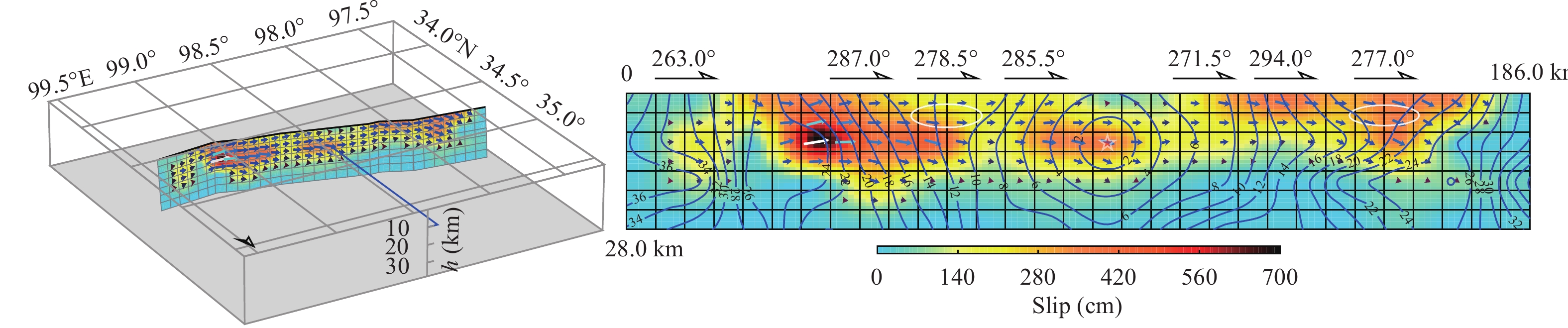
The source rupture model used in this paper was proposed by Wang WM et al. (2022) and was generated from joint inversion of seismic waveforms and InSAR coseismic displacement data. This study utilizes the source finite-fault model based on 7 fault planes with a width of 28 km and a dip of 84°, following Wang WM et al. (2022), as shown in Figure 2. Rupture propagated in both directions along the fault plane and produced 7 surface ruptures, which reached a total length of 186 km. The slip distribution of the Maduo earthquake presents three high-slip zones in the eastern, middle, and western parts of the fault plane. During the eastern propagation of the source rupture, a peak slip value of 682 cm occurred near 99°E, and the strike at the eastern end of the fault was deflected toward the north. During the western propagation of the source rupture, a peak slip value of 357 cm occurred near 97.8°E, and the strike at the western end of the fault was deflected towards the south (Wang WM et al., 2022). The detailed source fault parameters obtained by Wang WM et al. (2022) include the seismic moment of 2.27×10²⁰ N·m, which corresponds to a moment magnitude of 7.51, fault geometry (e.g., length, width, strike and dip), and rupture initiation point (hypocenter), as shown in Table 1.
Figure
2.
The temporal and spatial distributions of slip on the Maduo earthquake faults and a 3D view of the finite fault model from Wang WM et al. (2022). The chosen source model consists of 7 segments. Fault geometry and the detailed source time function of each subfault were employed in the simulation process.
Subsequently, to simulate the ground motion of the 2021 M7.4 Maduo earthquake, we utilized the Wang source rupture model from inversions instead of using the kinematic rupture model generated by the stochastic slip generator of Graves and Pitarka (2016). The Wang rupture model represents the overall rupture process of the earthquake, containing entire spatiotemporal evolutions of the rupture, such as the fault geometry, subfault size, rupture velocity, as well as the rise time, moment, and source time functions of each subfault.
2.3
Path model
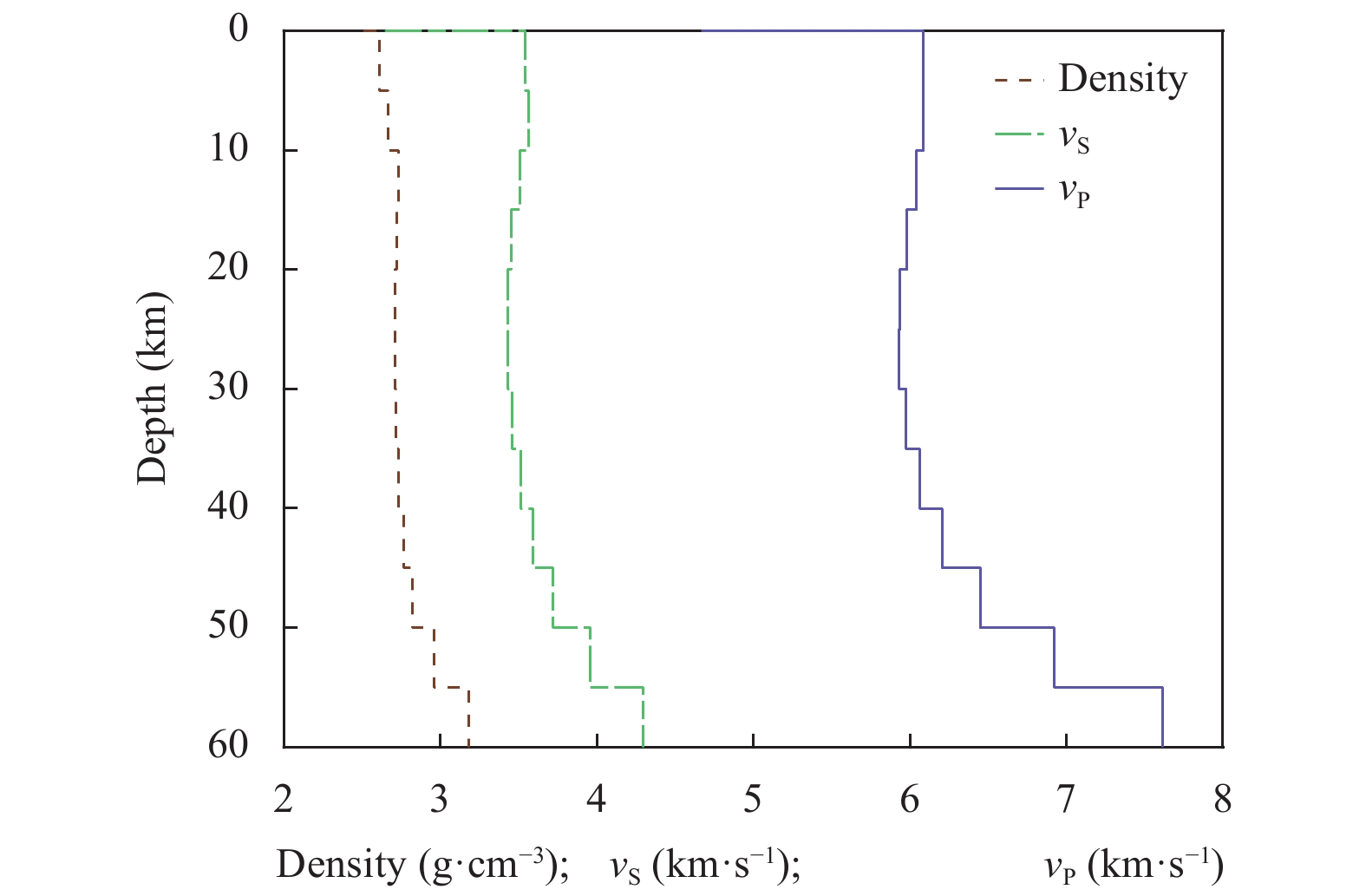
To incorporate the influence of the propagation path on the simulation results, we adopted the actual velocity model of the epicentral region of the M7.4 Maduo earthquake, which includes the influence of earth structure on ground motions. Xia SR et al. (2021) used the double-difference tomography method to image the 3D P- and S-wave velocity structures of the crust and upper mantle around the northeastern margin of the Tibetan Plateau. To simplify the calculation, we simplified the 3D velocity structure of the crust and upper mantle beneath the northeastern margin of the Tibetan Plateau into a 1D velocity model by averaging the P-wave velocity, S-wave velocity, and medium density at different depths, as shown in Figure 3.
Figure
3.
The 1D seismic velocity structure model (plotted as a function of depth) from Xia SR et al. (2021) which was used in our simulations. Continuous line represents P-wave speed, green dashed line is S-wave speed and purple dashed line is the density value.
During the Maduo earthquake, 16 strong-motion stations were triggered and recorded ground motions; 7 of these recordings were incomplete. Most of these observation stations are situated in the far-field region, more than 180 km from the epicenter, and these recordings have no engineering significance. Only stations 63DAW and 63XIH are located in the regional simulation domain illustrated in Figure 1, at distances of 175.47 km and 186.97 km from the epicenter, respectively. Nevertheless, the waveforms of all 16 distant stations illustrated in Figure 4 were simulated and validated against the observations. The epicentral distances of these stations are listed in Table 2.
Figure
4.
Locations of the 16 stations used for comparisons of waveforms and spectra. Bounding box (framed in green) indicates the study area in our research (the region shown in Figure 1). Fourteen strong motion stations are located outside of the near-fault region, while two strong motion stations (63DAW and 63XIH) are within the region used in the ground motion simulation.
The validation was conducted using the 16 strong motions available within 450 km of the epicenter. To prevent baseline drift and avoid loss of frequency information, the recordings were processed using the automatic baseline correction method proposed by Wang RJ et al. (2011). Figure 5 provides comparisons of the observed and simulated three-component acceleration broadband waveforms and their corresponding amplitudes at the 16 stations. Figure 6 provides comparisons of the observed and simulated three-component velocity broadband waveforms and amplitudes at the 16 stations. We found that the simulated amplitudes and durations of the three-component waveforms matched the recorded amplitudes and durations reasonably well at stations 63DAW and 63XIH. It should be noted that the PGA and PGV recorded at the other 14 stations were less than 10 cm/s2 and 5 cm/s, respectively. Although the simulated amplitudes are close to the recorded amplitudes, the effect of noise cannot be ignored. We noticed that recordings from 7 of the stations were incomplete. Comparisons of the duration time of shaking at the stations with missing partial recordings were not taken into account. Overall, a comparison of the waveforms reveals that the simulated waveforms are reasonably similar to the observed waveforms, in terms of amplitude and frequency. In general, the agreement between the simulated and observed waveforms is acceptable.
Figure
5.
Comparison of recorded (left) and simulated (right) broadband three-component ground acceleration waveforms at 16 sites around the earthquake. From top to bottom of each panel are the north-south (NS), east-west (EW), and up-down (UD) components. Station locations are indicated in Figure 4. The maximum value is listed above each waveform. Seven stations had incomplete recordings.
Figure
6.
Comparison of recorded (left) and simulated (right) broadband three-component ground velocity waveforms at 16 sites around the earthquake. From top to bottom of each panel are the north-south (NS), east-west (EW), and up-down (UD) components. The maximum value is listed above each waveform.
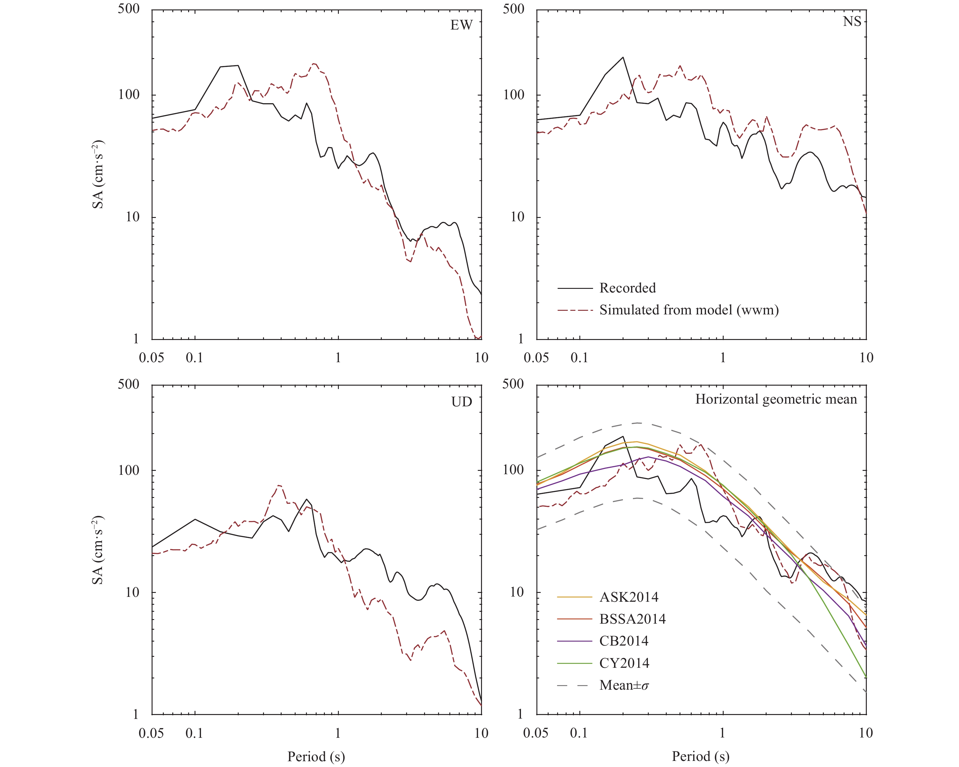
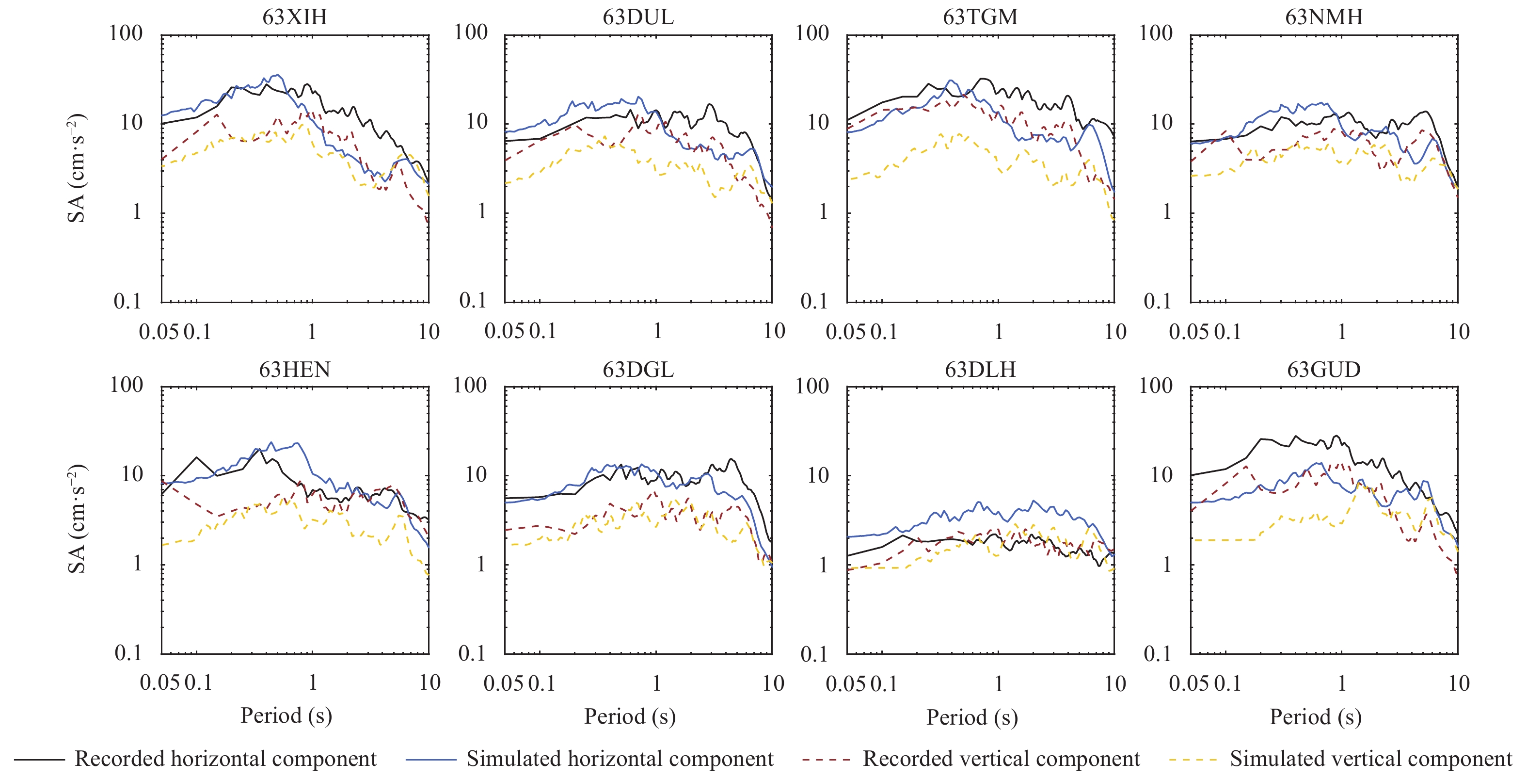
The SAs obtained from the recorded and simulated waveforms of station 63DAW were compared with the predictions from the NGA-West2 models, including the ASK2014 (Abrahamson et al., 2014), BSSA2014 (Boore et al., 2014), CB2014 (Campbell and Bozorgnia, 2014), and CY2014 (Chiou and Youngs, 2014) models. Figure 7 indicates that the simulated results are within one standard deviation of the predictions from the ground motion prediction equations (GMPEs), during the period of 0–10 s. The response spectra from simulated ground motions, the response spectra from recorded ground motions, and predicted response spectra at 63DAW are in good agreement. Horizontal and vertical recorded and simulated SA of another eight complete recording stations are plotted in Figure 8. The values of the acceleration response spectra of these stations were approximately an order of magnitude smaller than those of 63DAW.
Figure
7.
Comparison of the recorded (black solid lines) and simulated (red dotted lines) acceleration response spectra for 63DAW station and the predicted values of four NGA-West2 ground motion prediction equations (i.e. GMPEs) (colored lines). For comparison with the predictions of four NGA-West2 models, which only provide the average horizontal component of 5% damped linear pseudo-absolute acceleration response spectra, the recorded and simulated 5% damped pseudo-spectral acceleration was averaged horizontally (geometric mean) in the last sub-graph. The range indicated by the grey dashed lines represents the average value of the four NGA models ± 1 standard deviation σ.
Figure
8.
Comparisons of recorded and simulated acceleration response spectra from stations 63XIH, 63DUL, 63TGM, 63NMH, 63HEN, 63DGL, 63DLH, and 63GUD with horizontal geological mean (solid lines) and vertical (dashed lines) component. All are far-field stations.
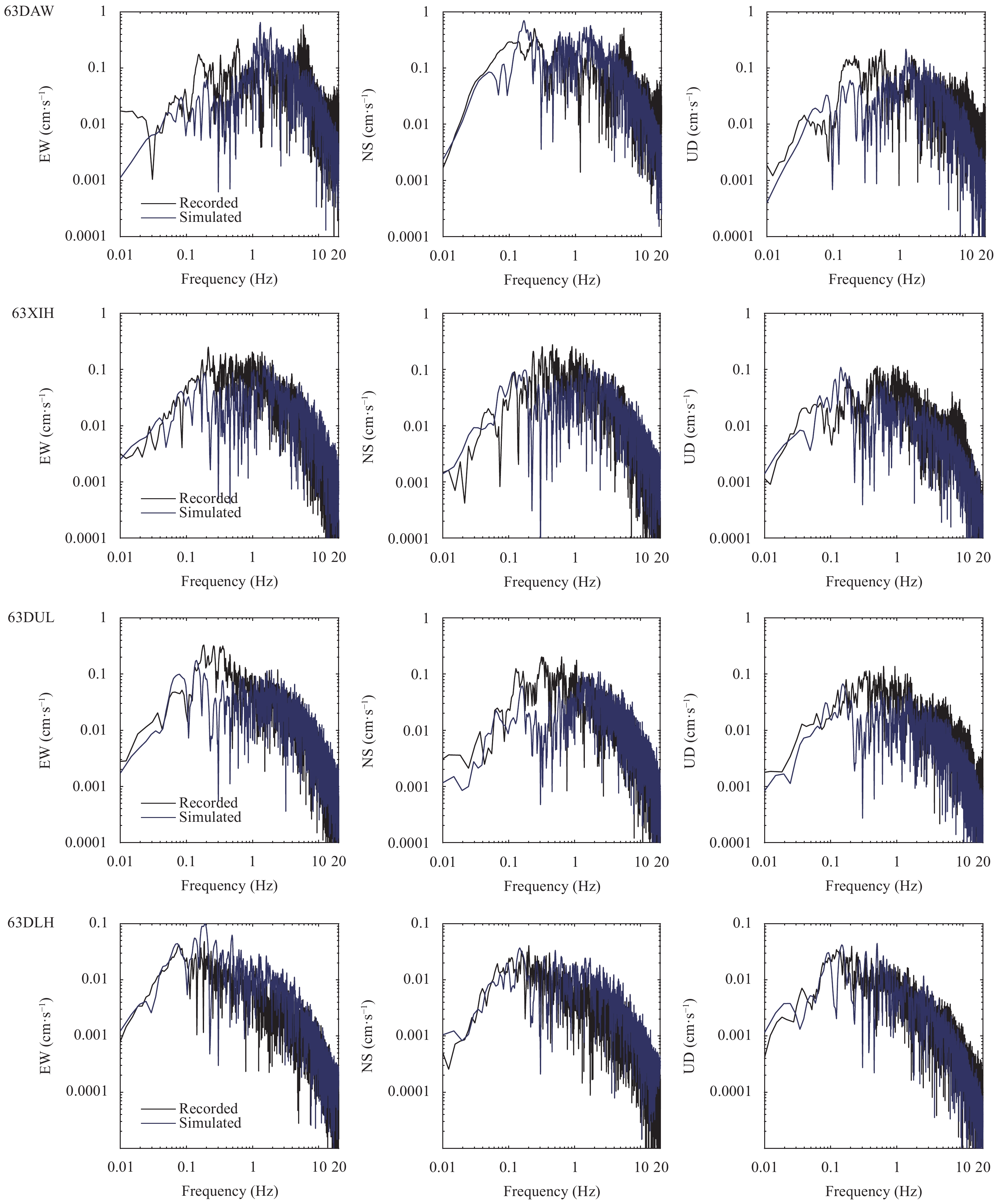
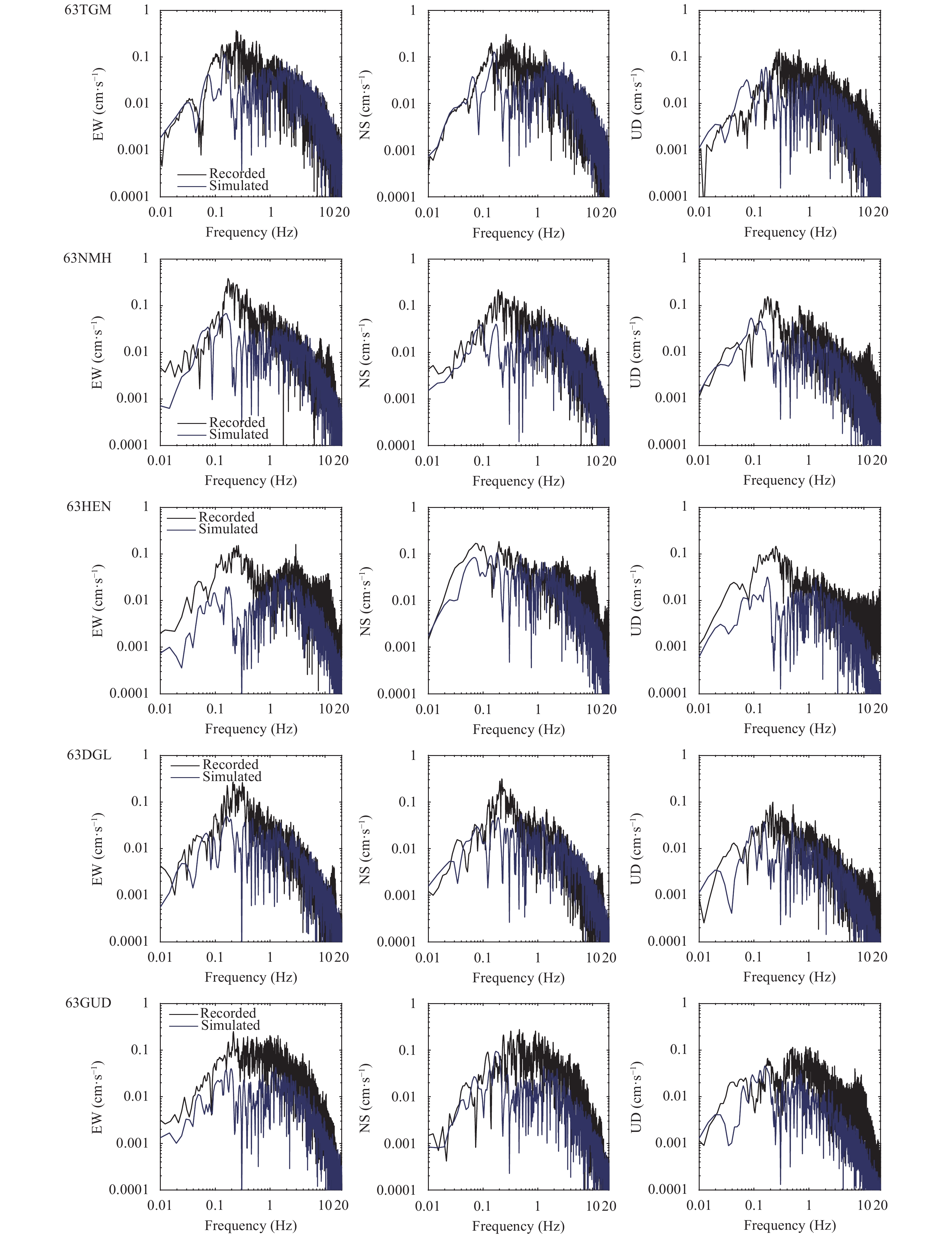
Figure 9 provides a comparison of the observed and simulated three-component Fourier amplitude spectra at stations 63DAW, 63XIH, 63DUL, and 63DLH. Both the level and trend of the observations were quite well matched by the simulations. Comparisons of the recorded and simulated three-component Fourier amplitude spectra at stations 63TGM, 63 NMH, 63HEN, 63DGL, and 63GUD are shown in Figure S1. In the high-frequency domain (greater than 1 Hz), the simulated Fourier amplitude spectra at most stations fit well with the recordings. We found that the simulation results underestimated the recorded values at 0.1–1 Hz at stations 63XIH and 63DUL. The absolute residuals of the Fourier amplitude spectra are small, showing little bias. The slight differences between the recorded and simulated Fourier amplitude spectra indicate that overall, the simulation could sufficiently reproduce the main characteristics of the ground motions observed during the Maduo earthquake.
Figure
9.
Comparison of recorded (black) and simulated (blue) Fourier amplitude spectra at stations 63DAW, 63XIH, 63DUL, and 63DLH. From left to right are the EW, NS, and UD components.
Strong ground motions were simulated in a regular 0.2°×0.2° grid covering the study area (96°E–101°E, 33°N–36°N). To capture the variation in near-field ground motions, we employed a refined 0.1°×0.1° grid immediately surrounding the fault (97°E–99.5°E, 34°N–35.3°N). The study area was divided into 38×22 latitudinal and longitudinal grids. In short, this process generated 897 intersections and endpoints, which were defined as sites for our simulation. The rupture fault, macroseismic intensity distribution, and strong ground motion stations in the study area are shown in Figure 1.
4.1
Attenuation of simulated ground motions and comparison with NGA-West2 models
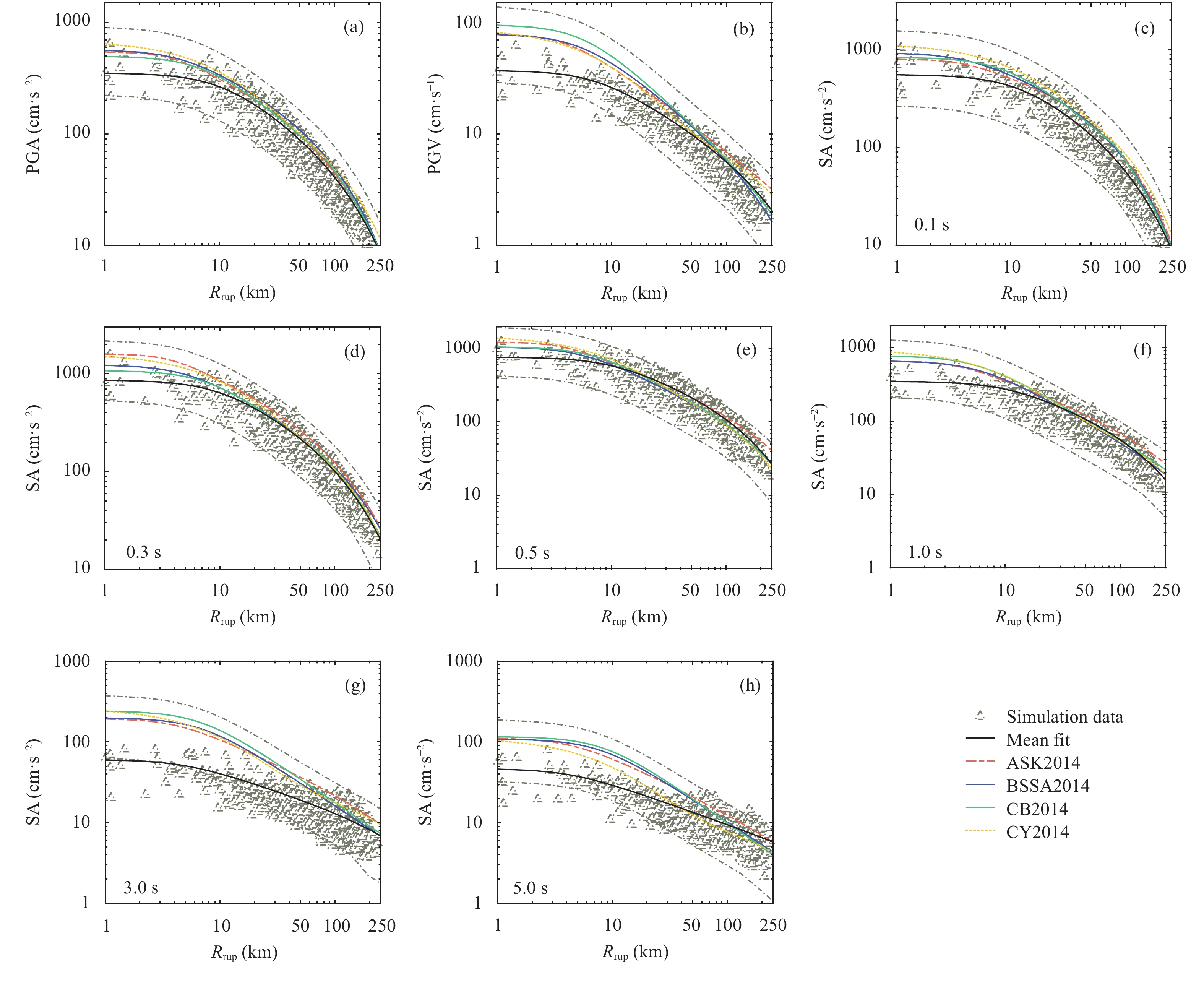
To evaluate the applicability of the NGA-West2 models to the simulated results, we compared the simulated results with predictions from the NGA-West2 models. Figure 10 shows the variations in three intensity measures (IMs), namely, the PGA, PGV, and SA at various periods (T = 0.1, 0.3, 0.5, 1.0, 3.0, and 5.0 s) for the simulated ground motions with the rupture distance (Rrup). These IMs are also compared with the values predicted by the NGA-West2 models. Based on the simulated results, we also developed a simplified ground motion model that includes both geometric and anelastic attenuation terms with rupture distance Rrup, as shown in Figure 10. The functional form, similar to the Campbell and Bozorgnia (2014) model, is given as
Figure
10.
Variations of the 897 simulated (a) PGAs, (b) PGVs, and 5% damped spectral acceleration at (c) 0.1 s, (d) 0.3 s, (e) 0.5 s, (f) 1.0 s, (g) 3.0 s, and (h) 5.0 s with rupture distance and the predicted attenuation of four NGA-West2 GMPEs. Open triangles indicate the horizontal averages of simulated intensity measures (IMs), black lines show the mean fit of 897 simulated results (coefficients of fit are provided in Table 3). Colored lines denote the four NGA models, dark dotted-dashed lines indicate the mean of the four NGA models ± 1 standard deviation σ.
where Y represents the intensity measures; a, b, c, and d are coefficients derived from least-squares regression analysis; and
σlnY is the standard deviation of the regression.
As shown in Figure 10a, c, d, e, and f, for PGA and SA values at short periods (T = 0.1, 0.3, 0.5, and 1.0 s), the median IM values fitted by simulations are slightly smaller than the median predictions from the four NGA-West2 models when Rrup ≤ 10 km. Nevertheless, when Rrup > 10 km, the median IM values fitted by simulations are more consistent with the median predictions. Overall, most of the simulated results fall within one standard deviation to either side of the values predicted by the four NGA-West2 models. However, Figure 10b, g, and h suggest that at longer periods (T = 3.0 s and 5.0 s), the fitted median simulated PGV and SA values are underestimated relative to the four NGA-West2 models over the whole distance range. The results suggest that the NGA-West2 models may not be suitable for describing ground motions for the long periods of the Maduo event, which occurred in the high-altitude hinterland of the eastern Tibetan Plateau.
Table
3.
Regression coefficients of PGA, PGV, and SA at period of 0.1 s, 0.3 s, 0.5 s, 1.0 s, 3.0 s and 5.0 s with source-to-site distance (Rrup) that fitted by 897 simulation results.
Coefficients
R2
σ
a
b
c
d
PGA
7.3130
−0.6644
9.608
−0.007
0.9276
0.2432
PGV
5.5020
−0.08627
8.32
0
0.8999
0.2171
SA (0.1 s)
8.2420
−0.7850
10.028
−0.0074
0.9353
0.2556
SA (0.3 s)
8.0130
−0.6026
9.201
−0.007
0.9151
0.2627
SA (0.5 s)
7.9870
−0.6223
9.193
−0.0062
0.8941
0.2731
SA (1.0 s)
7.6060
−0.6322
9.739
−0.0047
0.8748
0.2716
SA (3.0 s)
4.6060
−0.4655
4.68
−0.0014
0.6627
0.3254
SA (5.0 s)
4.3660
−0.4987
4.199
0
0.6967
0.2851
Note: R2 is a determination coefficient; σ signifies 1 standard deviation of the regression.
4.2
Regional features from spatial distributions of simulated intensity measures
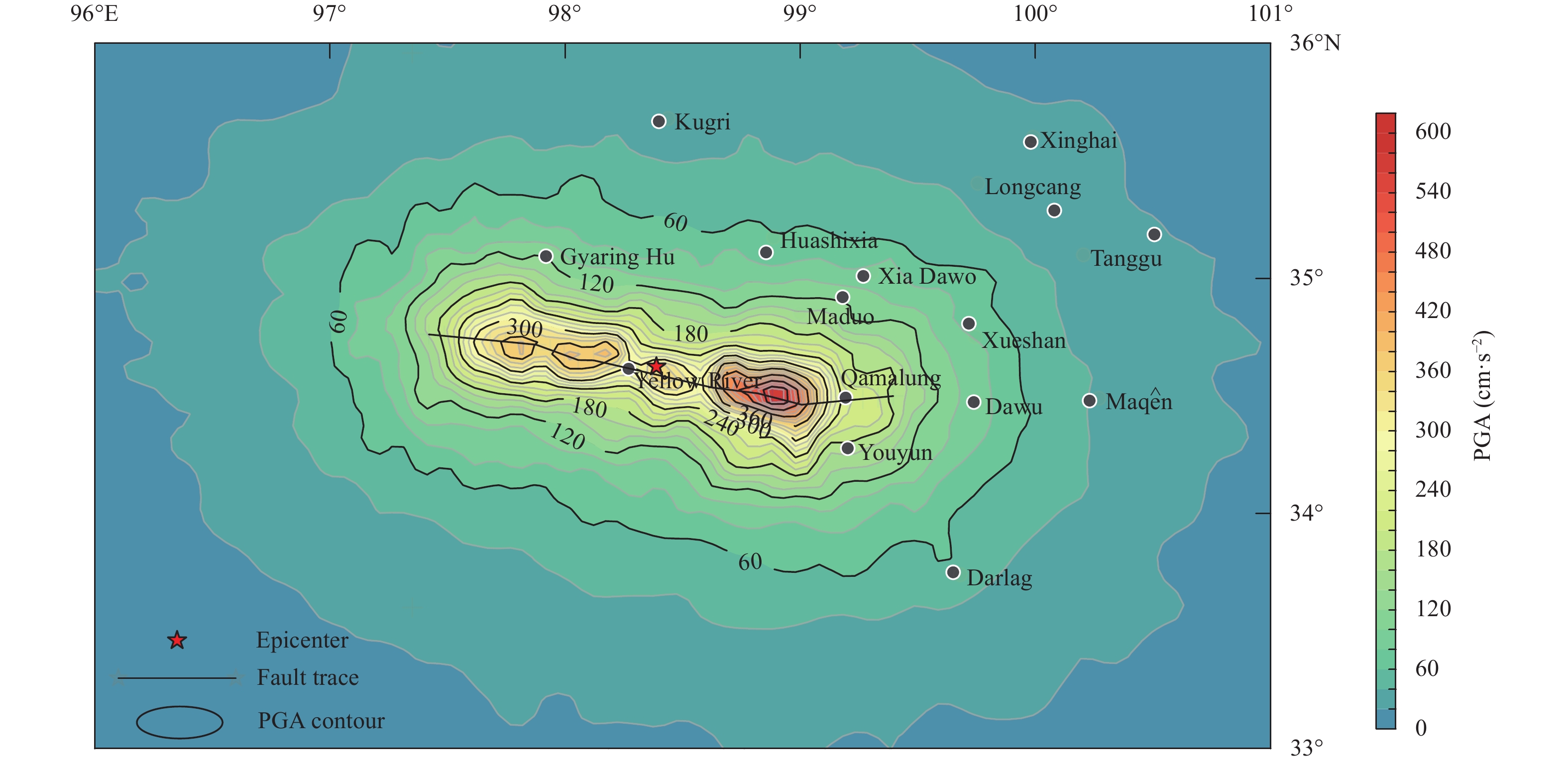
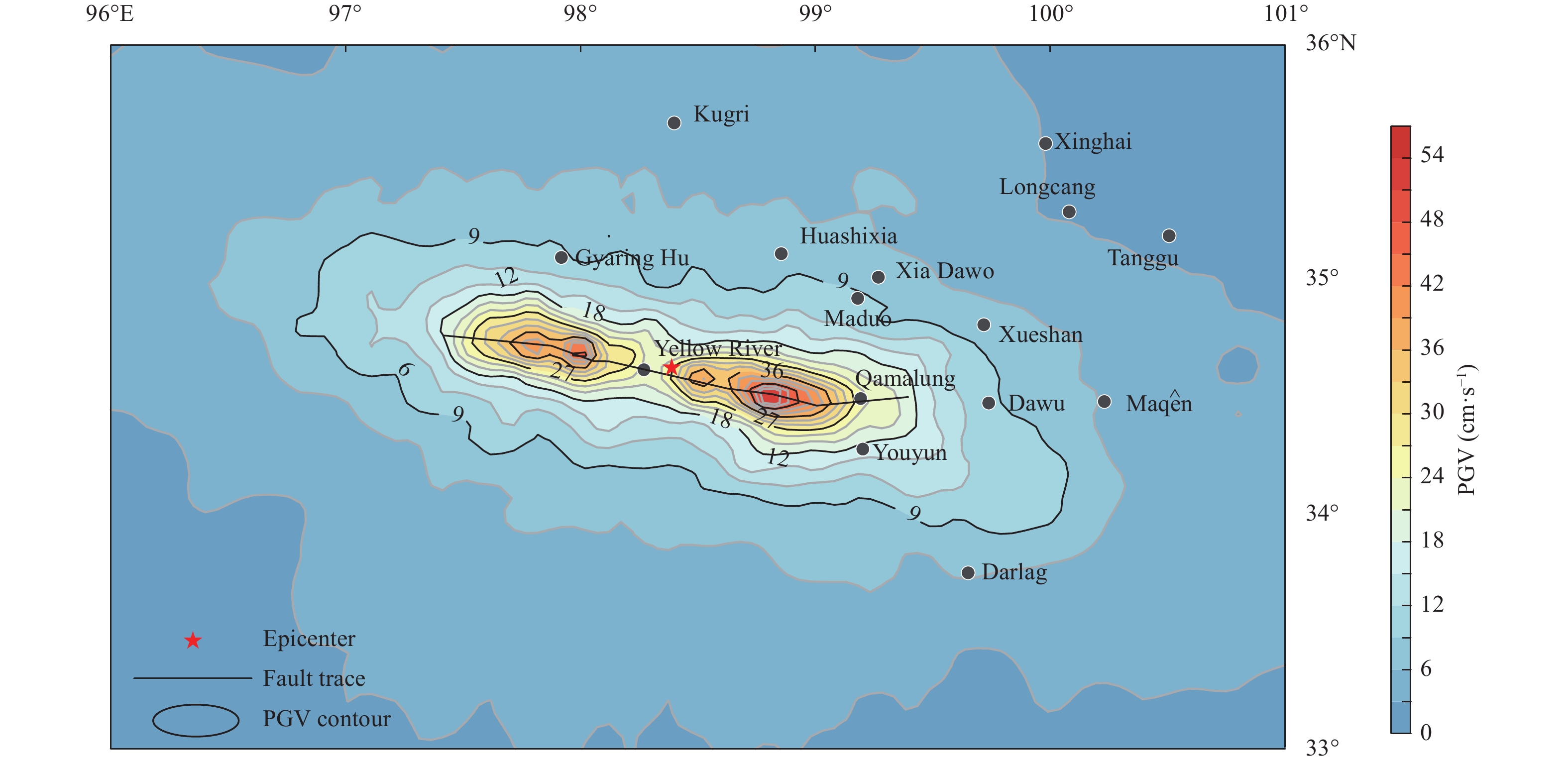
We investigated the spatial variation of the simulated PGA, PGV, and pseudo-spectral acceleration (PSA) at various periods (T = 0.1, 0.3, 0.5, 1.0, 3.0, and 5.0 s), as shown in Figures 11–13. The contours in these figures are elongated along the fault trace. Our simulations indicate that shaking intensity was significantly higher along the strike of the rupture and lower in the direction normal to the rupture, showing the significant rupture directivity effect. As can be seen from Figure 11, there are four concentrated areas with high PGA values in the gradient contour map. The location where the maximum PGA value reaches 575.26 cm/s2 is near the intersection of fault zones 6 and 7, rather than near the epicenter. Two regions with concentrated high PGV values can also be seen in Figure 12, near the intersection of fault segments 2 and 3 and the intersection of fault segments 5 and 6, with the maximum PGV reaching 45.42 cm/s. Figure 13 plots PSA distributions at various periods; the acceleration spectra corresponding to 0.1 s, 0.3 s, and 0.5 s are larger than those corresponding to 1.0 s, 3.0 s, and 5.0 s. Simulated PSA shows a relatively rapid attenuation with the period and weak dependence on the fault dimension. This indicates the high-frequency components of ground motions generated for the 2021 Maduo M7.4 earthquake using the GP method are more prominent than the low-frequency components. This result may be related to the multi-rupture fault model. Moreover, the low-frequency (long-period) PSA contours enclose a larger affected area than the high-frequency contours, extending from the near to middle-far field. Cao ZL et al. (2021) obtained similar results in the simulation of three-component ground motions of the Maduo earthquake. Nevertheless, we can infer from the simulation (Figure 11 to Figure 13) that the high-frequency ground motions are severely influenced by the details of the source rupture model, especially in the near-field region.
Figure
11.
Distribution of simulated PGA defined as the geometric mean of the north-south and east-west horizontal components. The gradient patterns were generated by applying natural neighbor interpolation to the 897 data points in the area. The numbers on each contour represent the PGA values in centimeters per square second.
Figure
13.
Distribution of simulated acceleration response spectra at periods (a) 0.1 s, (b) 0.3 s, (c) 0.5 s, (d) 1.0 s, (e) 3.0 s, and (f) 5.0 s, displayed as the horizontal average (geometric mean) component of 5% damped pseudo-spectral acceleration. The results were obtained by natural neighbor interpolation of 897 simulated values. The numbers on each contour denote the PSA values to corresponding period in the sub-graph, in units of centimeters per square second.
Figure
12.
Distribution of simulated PGV defined as the geometric mean of the north-south and east-west horizontal components. The numbers on each contour represent the PGV values in centimeters per second.
4.3
Simulated seismic intensity and comparison with macroseismic intensity
As mentioned previously, the shakemap of macroseismic intensity distribution for the Maduo earthquake is only an approximation, as it has very low resolution and large uncertainty in sparsely populated and high-altitude regions. Thus, the seismic intensity distributions were simulated and compared with the macroseismic intensities to overcome these shortcomings. We computed the seismic intensity from our simulations using the relationships between peak horizontal velocity, PGA, and modified Mercalli intensity (MMI) developed for shake maps (Wald et al., 1999, 2005). The functional form is given by Aagaard et al. (2008) as
Figure 14a displays the macroseismic intensity map issued by the Ministry of Emergency Management of the People′s Republic of China. Figure 14b displays a synthetic intensity map from simulations of the Maduo earthquake created with the Wang source model. The synthetic seismic intensities reveal a distribution of ground motion intensity with two regions of concentrated high values. Simulated seismic intensities were highest along the fault, especially where the estimated slip was high, and decreased rapidly along the direction perpendicular to strike. Figure 14c shows the intensity residuals between the synthetic intensity distribution and the reference macroseismic intensity distribution. These differences remain obvious. The misfit is largest in the far-field, where the evaluated intensities are at most two MMI units higher than the simulated intensities over significant areas. In most sites, the simulated intensity is 1 unit lower than the macroseismic intensity. Figure 14d shows a histogram of the difference between simulated and macroseismic intensities that approximately obeys the normal distribution and reveals a macroseismic intensity overestimation of one unit, with a mean residual of −0.87 and standard deviation of 0.53.
Figure
14.
Distribution of simulated modified Mercalli intensity (MMI) and numerical analysis of intensity residuals. Reference intensity distribution, provided by the Ministry of Emergency Management of the People′s Republic of China, is shown in (a); (b) and (c) are distributions of simulated MMI and the intensity residuals between simulations and the reference intensities. Intensity residuals of 897 sites are plotted as a histogram in (d); 95% confidence interval, the mean residual and standard deviation are displayed in the upper right corner.
We generated a map of intensity distribution within this region for the Maduo earthquake, based on multiple constraints including a detailed rupture model, regional velocity model with high resolution, and GP broadband simulation method. Thus, we assume that this map is more accurate than the macroseismic intensity map released by the Ministry of Emergency Management of the People′s Republic of China, with its low resolution and large uncertainties in high-altitude regions. A comparison of the two maps indicates that the latter tends to overestimate the ground shaking caused by the Maduo earthquake. The presented simulations provide ground motions that can be used to analyze the seismic performance of engineering structures in the 2021 Maduo earthquake.
4.4
Synthetic strong motion time histories at representative sites
It would be useful if ground motions could be deliberately simulated at selected sites that were lacking in ground motion records. In the Maduo region where ground motion recordings are sparse or non-existent, ground motion time histories are necessary for analyzing the structural seismic responses to this earthquake. The such analysis aids in estimating building damage and evaluating the performance of engineering structures at major damage sites. The 9 sites indicated in green in Figure 1 were chosen as a representative sample spanning the region covered by the simulation. Details of the locations of these sites are listed in Table 4. Figure 15 illustrates the three components of the simulated acceleration time histories, velocity time histories, and response spectra at the nine selected sites. The spatial variability of PGA and PGV at the selected sites was inspected. The sites A01, A02, A03, A04, and A05 near the faults were found to show larger amplitudes, whereas the sites A06, A07, A08, and A09 at a larger distance from the faults show lower-amplitude ground motions.
Table
4.
Information of representative sites in different seismic intensity regions which are marked as green triangles in Figure 1.
Site
Longitude (°E)
Latitude (°N)
Intensity
A01
98.00
34.70
X
A02
98.10
34.70
IX
A03
98.50
34.50
VIII
A04
97.70
34.80
VIII
A05
99.00
34.40
IX
A06
98.20
34.30
VII
A07
96.70
35.10
VI
A08
98.10
35.30
VI
A09
99.50
33.40
V
Note: The "Intensity" means the site locates in the corresponding intensity region which was released by the Ministry of Emergency Management of China in Figure 1.
Figure
15.
Three components of simulated acceleration time history (left), velocity time history (middle), and 5% damped response spectra (right) for the 9 representative sites listed in Table 4. The site number is indicated in the top left corner of each panel. Their locations are labeled in green in Figure 1. Of these sites, only A01 is located in the X intensity region. The durations of the acceleration and velocity waveforms are both 50 seconds, the maximum values are marked in the top-right corner of each panel.
These simulations can be directly used as ground motion inputs for dynamic analysis of forensic structural and geotechnical responses. During the earthquake, the Yematan Bridge (34.68°N, 98.06°E) and Yematan No. 2 Bridge (34.65°N, 98.04°E) on the Gongyu section of the Xili Expressway collapsed due to falling beams. The two bridges, located approximately 27 km from the epicenter between sites A01 and A02, experienced similar amplitudes and waveforms in the horizontal and vertical components. Based on these simulated results, we can infer that the Yematan Bridge and Yematan No. 2 Bridge suffered a peak acceleration of approximately 400 cm/s2 at ground level during the earthquake. Simulated time histories at the A01 and A02 sites can be used to analyze the damage to the two bridges and understand their seismic performance.
5.
Discussion
We restricted our broadband ground motion simulations to simplified wave propagation through a 1D-layered approximation of a 3D velocity model. The 1D layered region-specific velocity structure model was obtained from the local regional dataset and was used to calculate Green′s function, anelastic attenuation, and ground motion simulations for this earthquake. We recognize that the effects of surface topography were not considered, and our simulations do not take into account the effects of heterogenous 3D wave propagation, which modulate the resulting ground shaking levels and their distributions. Unfortunately, detailed 3D crustal models are limited to a few small areas worldwide and commonly suffer from limited spatial resolution (Imperatori and Mai, 2012). Modeling of complex wave propagation phenomena associated with the 3D structure of this region may require further explicit inclusion of surface topography effects in the numerical simulation GP method for regional ground motion simulation.
6.
Summary and conclusions
Combining the kinematic source model of the 2021 Maduo M7.4 earthquake from Wang WM et al. (2022) with a high-resolution regional seismic velocity model allowed for the successful simulation of primary spatial variations in shaking intensity. The simulated data showed good agreement with the data recorded at station 63DAW, indicating that simulations of this event could be used to study the ground motion characteristics in the near-fault region. The waveforms, acceleration response spectra, and Fourier amplitude spectra at triggered strong motion stations were used to validate the observations. The simulations provided a reasonable fit for the observations. In general, the agreement between observations and simulations is acceptable. Ground motions were simulated at 897 virtual grid stations in the epicentral region and presented as PGA, PGV, and SA contour plots. In addition, the acceleration and velocity time histories and response spectra were provided for the selected representative sites where no strong motion recordings were available. Our results indicate that the officially released macroseismic intensities for the 2021 Maduo earthquake have large uncertainties in sparsely populated high-altitude regions and the ground shakings are generally overestimated by an average of one MMI unit in most sites of the epicenter region. The spatial distributions of PGA, PGV, SA, and MMI in the near-field region reveal two relatively high-value concentrations that correspond to the surface projection of the high-slip area on the fault plane, indicating the dominant effect of the source rupture model in the near-field simulation. Moreover, the results suggest uneven distributions of PGA, PGV, and SA, reflecting the complexity of the source rupture model. Our simulations show that the high-frequency components of ground motions were prominent, while the low-frequency components were not. This phenomenon is unexpected for large earthquakes and may be related to the multi-segment fault rupture caused by this large earthquake. Our research suggests that the four NGA-West2 models are effective at describing ground motions for short periods. However, NGA-West2 models are not suitable for describing ground motions for the long periods of the Maduo event, which occurred in the high-altitude hinterland of the eastern Tibetan Plateau.
We conclude that in light of recent knowledge of the source rupture model, regional and local velocity structure, and hybrid broadband ground motion simulation techniques, our simulation of the 2021 Maduo earthquake ground motions has yielded reliable and useful results. Hence, the simulated results have important implications for evaluating the performance of engineering structures in the epicentral regions of this earthquake and for estimating seismic hazards in the Tibetan regions where no strong ground motion records of large earthquakes are available. Similarly, these simulated results can provide data support for refining macroseismic intensity maps in sparsely populated areas with few buildings.
Supporting Information
Figure
S1.
Recorded (black) and simulated (blue) three-component Fourier spectra for stations 63TGM, 63NMH, 63HEN, 63DGL, and 63GUD.
The authors thank the National Strong-Motion Observation Network System (NSMONS) of China for providing the strong motion data for the Maduo M7.4 earthquake. We appreciate the detailed explanation of the source rupture process provided by Prof. Weimin Wang. We would like to thank Prof. Yonghua Li and Dr. Lei Shi for providing the digital 3D model of the velocity structure of the crust and upper mantle beneath the northeastern margin of the Tibetan Plateau. The authors thank Graves and Pitarka for making their code, relating to broadband ground motion simulation, available online. The authors also thank Prof. Yongge Wan for his help. The constructive reviews provided by all anonymous reviewers were very helpful in revising the paper. Financial support for this study was provided by the National Key Research and Development Project (No. 2020YFA0710603) and the Special Fund of the Institute Geophysics, China Earthquake Administration (No. DQJB22B27).
Aagaard BT, Brocher TM, Dolenc D, Dreger D, Graves RW, Harmsen S, Hartzell S, Larsen S and Zoback ML (2008). Ground-motion modeling of the 1906 San Francisco earthquake, part I: Validation using the 1989 Loma Prieta earthquake. Bull Seismol Soc Am 98(2): 989– 1011 https://doi.org/10.1785/0120060409.
Abrahamson NA, Silva WJ and Kamai R (2014). Summary of the ASK14 ground motion relation for active crustal regions. Earthq Spectra 30(3): 1025 – 1055 https://doi.org/10.1193/070913EQS198M.
Beresnev IA and Atkinson GM (1997). Modeling finite-fault radiation from the ωn spectrum. Bull Seismol Soc Am 87(1): 67 – 84 https://doi.org/10.1785/BSSA0870010067.
Boore DM (2003). Simulation of ground motion using the stochastic method. Pure Appl Geophys 160(3–4): 635 – 676 https://doi.org/10.1007/PL00012553.
Boore DM, Stewart JP, Seyhan E and Atkinson GM (2014). NGA-West2 equations for predicting PGA, PGV, and 5% damped PSA for shallow crustal earthquakes. Earthq Spectra 30(3): 1057 – 1085 https://doi.org/10.1193/070113EQS184M.
Campbell KW and Bozorgnia Y (2014). NGA-West2 ground motion model for the average horizontal components of PGA, PGV, and 5% damped linear acceleration response spectra. Earthq Spectra 30(3): 1087 – 1115 https://doi.org/10.1193/062913EQS175M.
Cao ZL, Tao XX and Tao ZR (2021). Simulation of three-component near-fault ground motions during the 2021 Maduo M7.4 earthquake. World Earthq Eng 37(4): 1 – 11 https://doi.org/10.3969/j.issn.1007-6069.2021.04.001 (in Chinese with English abstract).
Chen KJ, Avouac JP, Geng JH, Liang CR, Zhang ZG, Li ZC and Zhang SP (2022). The 2021 MW7.4 Madoi Earthquake: An archetype bilateral slip-pulse rupture arrested at a splay fault. Geophys Res Lett 49(2): e2021GL095243 https://doi.org/10.1029/2021GL095243.
Chiou BSJ and Youngs RR (2014). Update of the Chiou and Youngs NGA model for the average horizontal component of peak ground motion and response spectra. Earthq Spectra 30(3): 1117 – 1153 https://doi.org/10.1193/072813EQS219M.
Day SM and Bradley CR (2001). Memory-efficient simulation of anelastic wave propagation. Bull Seismol Soc Am 91(3): 520 – 531 https://doi.org/10.1785/0120000103.
Graves R and Pitarka A (2004). Broadband time history simulation using a hybrid approach. In: 13th World Conference on Earthquake Engineering. Vancouver, BC, Canada.
Graves R and Pitarka A (2016). Kinematic ground-motion simulations on rough faults including effects of 3D stochastic velocity perturbations. Bull Seismol Soc Am 106(5): 2136 – 2153 https://doi.org/10.1785/0120160088.
Graves RW (1996). Simulating seismic wave propagation in 3D elastic media using staggered-grid finite differences. Bull Seismol Soc Am 86(4): 1091– 1106.
Graves RW, Aagaard BT, Hudnut KW, Star LM, Stewart JP and Jordan TH (2008). Broadband simulations for MW 7.8 southern San Andreas earthquakes: Ground motion sensitivity to rupture speed. Geophys Res Lett 35(22): L22302 https://doi.org/10.1029/2008GL035750.
Graves RW and Pitarka A (2010). Broadband ground-motion simulation using a hybrid approach. Bull Seismol Soc Am 100(5A): 2095 – 2123 https://doi.org/10.1785/0120100057.
Hartzell S, Harmsen S, Frankel A and Larsen S (1999). Calculation of broadband time histories of ground motion: Comparison of methods and validation using strong-ground motion from the 1994 Northridge earthquake. Bull Seismol Soc Am 89(6): 1484 – 1504 https://doi.org/10.1785/BSSA0890061484.
Hough SE and Graves RW (2020). The 1933 Long Beach Earthquake (California, USA): Ground motions and rupture scenario. Sci Rep 10(1): 10017 https://doi.org/10.1038/s41598-020-66299-w.
Imperatori W and Mai PM (2012). Sensitivity of broad-band ground-motion simulations to earthquake source and Earth structure variations: an application to the Messina Straits (Italy). Geophys J Int 188(3): 1103 – 1116 https://doi.org/10.1111/j.1365-246X.2011.05296.x.
Lee WHK, Kanamori H, Jennings PC and Kisslinger C (2003). International Handbook of Earthquake and Engineering Seismology. International Geophysics (Vol. 81, Part B). Academic Press, New York, pp 937–1948.
Li Q, Wan YG, Li CT, Tang H, Tan K and Wang DZ (2022). Source process featuring asymmetric rupture velocities of the 2021 MW7.4 Maduo, China, Earthquake from teleseismic and geodetic data. Seismol Res Lett 93(3): 1429 – 1439 https://doi.org/10.1785/0220210300.
Liu CY, Bai L, Hong SY, Dong YF, Jiang Y, Li HR, Zhan HL and Chen ZW (2021). Coseismic deformation of the 2021 MW7.4 Maduo earthquake from joint inversion of InSAR, GPS, and teleseismic data. Earthq Sci 34(5): 436 – 446 https://doi.org/10.29382/eqs-2021-0050.
Lyu MZ, Chen KJ, Xue CH, Zang N, Zhang W and Wei GG (2022). Overall subshear but locally supershear rupture of the 2021 MW7.4 Maduo earthquake from high-rate GNSS waveforms and three-dimensional InSAR deformation. Tectonophysics 839: 229542 https://doi.org/10.1016/j.tecto.2022.229542.
Pitarka A (1999). 3D elastic finite-difference modeling of seismic motion using staggered grids with nonuniform spacing. Bull Seismol Soc Am 89(1): 54– 68 https://doi.org/10.1785/BSSA0890010054.
Pitarka A, Graves R, Irikura K, Miyakoshi K, Wu CJ, Kawase H, Rodgers A and McCallen D (2021). Refinements to the Graves-Pitarka kinematic rupture generator, including a dynamically consistent slip-rate function, applied to the 2019 MW 7.1 ridgecrest earthquake. Bull Seismol Soc Am 112(1): 287– 306 https://doi.org/10.1785/0120210138.
Razafindrakoto HNT, Bradley BA and Graves RW (2018). Broadband ground-motion simulation of the 2011 MW 6.2 Christchurch, New Zealand, Earthquake. Bull Seismol Soc Am 108(4): 2130 – 2147 https://doi.org/10.1785/0120170388.
Ren JJ, Xu XW, Zhang GW, Wang QX, Zhang ZW, Gai HL and Kang WJ (2022). Coseismic surface ruptures, slip distribution, and 3D seismogenic fault for the 2021 MW7.3 Maduo earthquake, central Tibetan Plateau, and its tectonic implications. Tectonophysics 827: 229275 https://doi.org/10.1016/j.tecto.2022.229275.
Wald DJ, Quitoriano V, Heaton TH, Kanamori H, Scrivner CW and Worden CB (1999). TriNet “ShakeMaps”: Rapid generation of peak ground motion and intensity maps for earthquakes in southern California. Earthq Spectra 15(3): 537– 555 https://doi.org/10.1193/1.1586057.
Wald DJ, Worden BC, Quitoriano V and Pankow KL (2005). ShakeMap® manual: Technical manual, users guide, and software guide (Version 1.0). U. S. Geol Surv Tech Meth. , 12-A1, 132. https://pubs.usgs.gov/tm/2005/12A01/pdf/508TM12-A1.pdf
Wang RJ, Schurr B, Milkereit C, Shao ZG and Jin MP (2011). An improved automatic scheme for empirical baseline correction of digital strong-motion records. Bull Seismol Soc Am 101(5): 2029 – 2044 https://doi.org/10.1785/0120110039.
Wang WM, He JK, Wang X, Zhou Y, Hao JL, Zhao LF and Yao ZX (2022). Rupture process models of the Yangbi and Maduo earthquakes that struck the eastern Tibetan Plateau in May 2021. Sci Bull 67(5): 466 – 469 https://doi.org/10.1016/j.scib.2021.11.009.
Xia SR, Shi L, Li YH and Guo LH (2021). Velocity structures of the crust and uppermost mantle beneath the northeastern margin of Tibetan plateau revealed by double-difference tomography. Chin J Geophys 64(9): 3194 – 3206 https://doi.org/10.6038/cjg2021O0514 (in Chinese with English abstract).
Yue H, Shen ZK, Zhao ZY, Wang T, Cao BN, Li Z, Bao XW, Zhao L, Song XD, Ge ZX, Ren CM, Lu WF, Zhang Y, Liu-Zeng J, Wang M, Huang QH, Zhou SY and Xue L (2022). Rupture process of the 2021 M7.4 Maduo earthquake and implication for deformation mode of the Songpan-Ganzi terrane in Tibetan Plateau. Proc Natl Acad Sci USA 119(23): e2116445119 https://doi.org/10.1073/pnas.2116445119.
Zhang X, Feng WP, Du HL, Samsonov S and Yi L (2022). Supershear rupture during the 2021 MW 7.4 Maduo, China, earthquake. Geophys Res Lett 49(6): e2022GL097984 https://doi.org/10.1029/2022GL097984.
Table
3.
Regression coefficients of PGA, PGV, and SA at period of 0.1 s, 0.3 s, 0.5 s, 1.0 s, 3.0 s and 5.0 s with source-to-site distance (Rrup) that fitted by 897 simulation results.
Coefficients
R2
σ
a
b
c
d
PGA
7.3130
−0.6644
9.608
−0.007
0.9276
0.2432
PGV
5.5020
−0.08627
8.32
0
0.8999
0.2171
SA (0.1 s)
8.2420
−0.7850
10.028
−0.0074
0.9353
0.2556
SA (0.3 s)
8.0130
−0.6026
9.201
−0.007
0.9151
0.2627
SA (0.5 s)
7.9870
−0.6223
9.193
−0.0062
0.8941
0.2731
SA (1.0 s)
7.6060
−0.6322
9.739
−0.0047
0.8748
0.2716
SA (3.0 s)
4.6060
−0.4655
4.68
−0.0014
0.6627
0.3254
SA (5.0 s)
4.3660
−0.4987
4.199
0
0.6967
0.2851
Note: R2 is a determination coefficient; σ signifies 1 standard deviation of the regression.
Table
4.
Information of representative sites in different seismic intensity regions which are marked as green triangles in Figure 1.
Site
Longitude (°E)
Latitude (°N)
Intensity
A01
98.00
34.70
X
A02
98.10
34.70
IX
A03
98.50
34.50
VIII
A04
97.70
34.80
VIII
A05
99.00
34.40
IX
A06
98.20
34.30
VII
A07
96.70
35.10
VI
A08
98.10
35.30
VI
A09
99.50
33.40
V
Note: The "Intensity" means the site locates in the corresponding intensity region which was released by the Ministry of Emergency Management of China in Figure 1.

 DownLoad: