A review of the influencing factors on teleseismic traveltime tomography

1.   Introduction

Seismic traveltime tomography is a powerful tool to detect the Earth′s interior (Rawlinson et al., 2010; Foulger et al., 2013; Zhao DP et al., 2013). Since 1976, many studies on seismic traveltime tomography have been made (Aki and Lee, 1976; Aki et al., 1977; Dziewonski, 1984; Zhao DP et al., 1994; Zhang HJ and Thurber, 2006; Tong P et al., 2014; Liu SL et al., 2019; Lei WJ et al., 2020; Bai T et al., 2020). Seismic traveltime tomography has been successfully implemented in areas with various scales, such as local (Bai T et al., 2020), regional (Huang ZC et al., 2015) and global scales (Lei WJ et al., 2020). For the tomography model with local or regional scale, teleseismic earthquakes can be used for study. This kind of tomography is called teleseismic traveltime tomography (Aki et al., 1977; Rawlinson et al., 2010; Lei JS and Zhao DP, 2016; Yao JY et al., 2021). Because seismic rays from teleseismic events can sample the deep part of model, teleseismic traveltime tomography is able to resolve structures at great depths (Liu SL et al., 2021; Yao JY et al., 2021).

The fundamental assumption of teleseismic traveltime tomography is that hypocentral uncertainties and global mantle heterogeneities outside the target imaging domain do not significantly affect the imaging results (Aki et al., 1977; Zhao DP et al., 1994; Masson and Trampert, 1997; Rawlinson et al., 2006). Although this assumption is widely accepted in tomographic studies, special considerations should be evaluated. For example, according to Masson and Trampert (1997), Zhao DP et al. (2013) and Lei JS and Zhao DP (2016), the influences of global mantle heterogeneities cannot be ignored in some cases, and heterogeneities outside the imaging domain may modify the amplitudes of relative velocity anomalies. Moreover, although the influences of mantle heterogeneities have been investigated by a few researchers (Foulger et al., 2013; Lei JS and Zhao DP, 2016; Masson and Trampert, 1997; Zhao DP et al., 2013), other influencing factors, such as measurements for relative traveltime differences, station spacings and source uncertainties, have seldom been studied.

In teleseismic traveltime tomography, the absolute traveltime is not directly inverted because it is sensitive to global mantle heterogeneities and source uncertainties (Aki et al., 1977; Yuan YO et al., 2016). However, the effects of global mantle heterogeneities and source uncertainties are reduced by relative traveltime differences because the rays for conducting relative traveltime differences share the same teleseismic source and ray paths outside the imaging domain are close to each other (Zhao DP et al., 2013). Thus, to satisfy the abovementioned fundamental assumption for teleseismic traveltime tomography, two methods have been proposed to measure relative traveltime differences: one (hereafter named M1) calculates the relative traveltime difference between two adjacent stations (Liu SL et al., 2018) and the other (named M2) is achieved by subtracting the average traveltime of all stations from the traveltime of each station (Aki et al., 1977; Rawlinson et al., 2006).

In this review, we further discuss the influencing factors on teleseismic traveltime tomography through synthetic data analyses and imaging examples. Specifically, the influencing factors discussed in this article include the methods for measuring relative traveltime differences, the presence of global mantle heterogeneities, the station spacing and the uncertainties in teleseismic event locations. Although some researchers have investigated the influence of mantle heterogeneities on teleseismic tomography with M2 (Foulger et al., 2013), comprehensive insights have not been offered into the other influences. Moreover, although some qualitative studies have examined the influences of station spacings and source uncertainties (Aki et al., 1977; Liu SL et al., 2021), a quantitative investigation is lacking. Therefore, an integral study of these influencing factors is necessary, which may provide some guidelines for teleseismic traveltime tomography in practical applications.

2.   Method

In seismic tomography, relative traveltime differences are generally measured to reduce model and source uncertainties (Aki et al., 1977; Zhang HJ et al., 2017). In particular, two measurement methods, M1 and M2, are adopted in teleseismic traveltime tomography. For M1, the traveltime difference ${t}_{jk}^{i}$ between the j- and k-th stations for the i-th event can be expressed as:

where T is the observed or calculated traveltime at a given station. Here, the two adjacent stations, j- and k-stations, form a station pair. Based on Equation (1), the residual ${r}_{jk}^{i}$ (the difference between the observed and calculated traveltime differences) can be written as:

where the superscripts obs and cal denote the observed and calculated traveltimes, respectively. The measurement formulated in Equation (2) can be incorporated for teleseismic traveltime tomography. For M2, the relative traveltime difference ${t}_{j}^{i}$ evaluated at thej-th station for the i-th event is computed by the following formula:

where ${{\bar{T}}^{i}}=\dfrac{1}{m}\mathop\sum\limits_{j=1}^{m}{T_{j}^{i}}$ is the average traveltime over all m stations. The residual ${r}_{j}^{i}$ (the difference between the observed and calculated relative traveltime differences) is given by:

The measurement described in Equation (4) is frequently employed for teleseismic traveltime tomography. In practice, the relative traveltime differences in Equations (2) and (4) can be computed using cross-correlation methods (Rawlinson et al., 2006; Liu SL et al., 2018). They can also be calculated after hand-picking the arrivals (Zhao DP et al., 1994; Lei JS and Zhao DP, 2016).

Synthetic tests are an effective tool to investigate influencing factors (Masson and Trampert, 1997; Zhao DP et al., 2013). Zhao DP et al. (2013) used the 3-D ray tracing technique, which combines the pseudo-bending method with Snell′s law, to calculate the ray paths and traveltimes for synthetic tests. Here, we use the fast marching method (FMM) (Sethian and Popovici, 1999; Rawlinson and Sambridge, 2004, 2005) to compute ray paths and traveltimes. According to Liu YS and Tong P (2021), the FMM is able to more accurately determine the ray paths and traveltimes in a strong heterogeneous model than the conventional pseudo-bending method.

For a synthetic inversion, the velocities in the target volume are obtained by solving the following damped least-square problem:

where A is the sensitivity matrix; X is the vector composed of model perturbation; ${\bf{C}}_{\mathrm{d}}$ is the a priori data covariance matrix; ${\bf{C}}_{\mathrm{m}}$ is the a priori model covariance matrix; η is the damping factor; b contains the differential relative traveltime data (Liu SL et al., 2018, 2021; Yao JY et al., 2021; Li MY et al., 2022). The inversion process consists of three steps. The first step is the construction of an initial model. We choose the ak135 stratified Earth model (Kennett et al., 1995) as the initial model in this study. The second step is the calculation of differential relative traveltime data using the FMM. The third step is the inversion of velocity model using the conjugate gradient method (Hestenes and Stiefel, 1952; Tong P et al., 2014). To steadily update the model, a prescribed level is set to constrain the maximum relative perturbation at each iteration by adjusting the damping factor (Liu SL et al., 2018).

3.   Study area

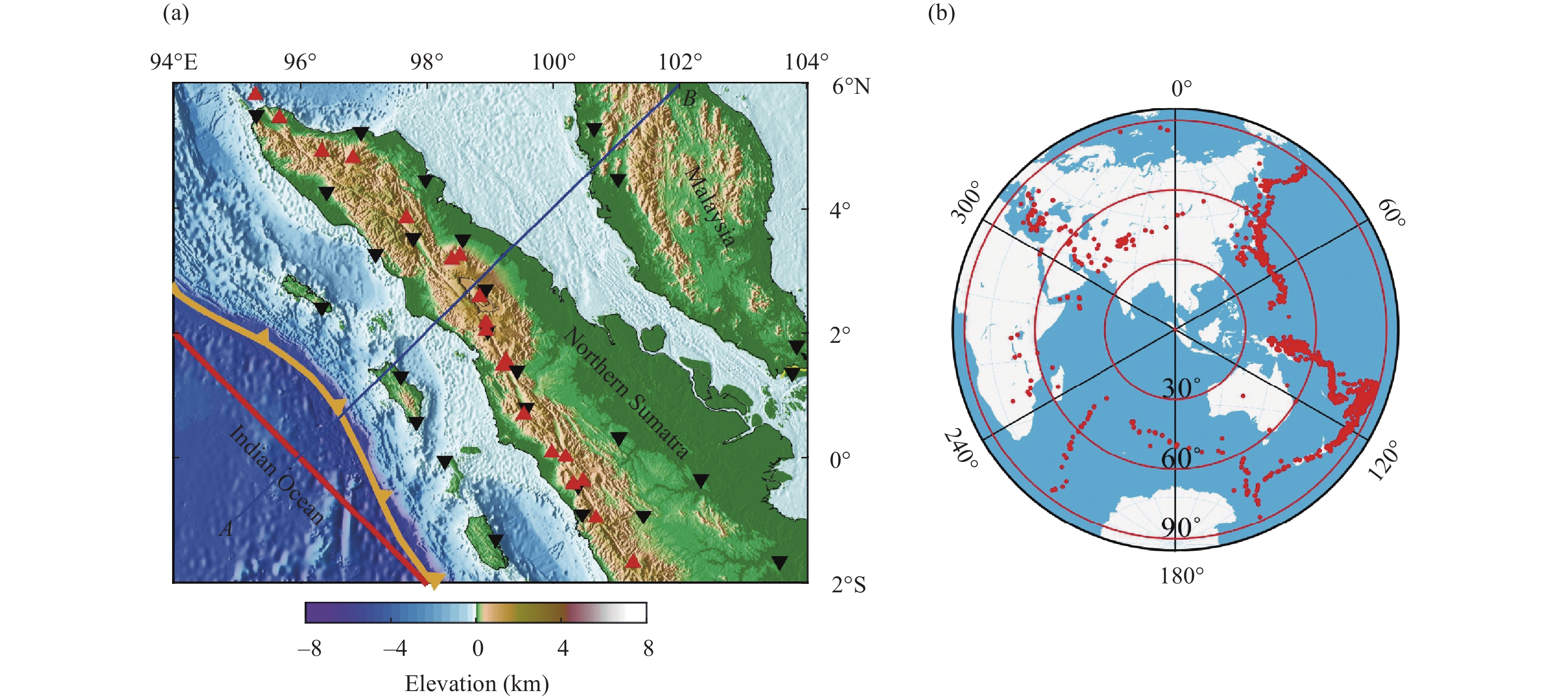
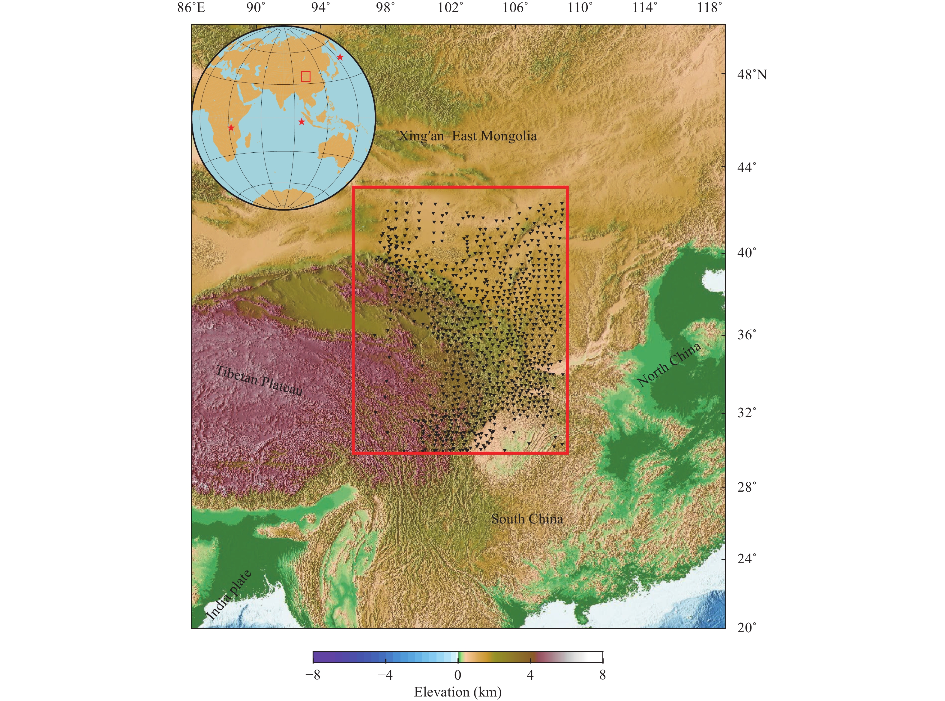
To analyze the influencing factors of teleseismic traveltime tomography, we select the NE Tibetan Plateau (96°E–109°E, 30°N–43°N) as the study area for synthetic data analyses and imaging examples. In the area, a total of 927 stations (Figure 1) (Li MY et al., 2022) with an average lateral spacing of 0.5° are available for teleseismic tomography. The stations were employed by Li MY et al. (2022) to image the crust and mantle structures in the NE Tibetan Plateau. The relatively even deployment of these stations greatly avoids the uneven distribution of station pairs when the M1 is used for measurement. In the main text, we investigate the influences mainly based on the study of the NE Tibetan Plateau. To further analyze the influences, another study area (Figure S1 in the Supplementary information), i.e., northern Sumatra (94°E–104°E, 2°S–6°N), is also employed for discussion.

4.   Four influencing factors on teleseismic traveltime tomography

4.1   Influence of the two measurement methods

Both M1 and M2 have been extensively used to resolve the interior structures of the Earth (Aki et al., 1977; Lei JS and Zhao DP, 2016; Civiero et al., 2018; Song JH et al., 2018; Yao JY et al., 2021; Liu SL et al., 2021; Li MY et al., 2022). Aki et al. (1977), Rawlinson et al. (2006) and Zhao DP et al. (2013) pointed out that M2 can remove the errors from source origin time and hypocenter location and minimize the effects of mantle heterogeneities. Liu SL et al. (2018, 2021) considered that M1 is an alterative efficient method for teleseismic tomography. Robust imaging results are obtained by using M1 (Liu SL et al., 2018, 2021; Yao JY et al., 2021). However, the advantages and disadvantages of M1 and M2 is seldomly mentioned. Here, we conduct a thorough study of the two measurement methods (M1 and M2) through synthetic tests.

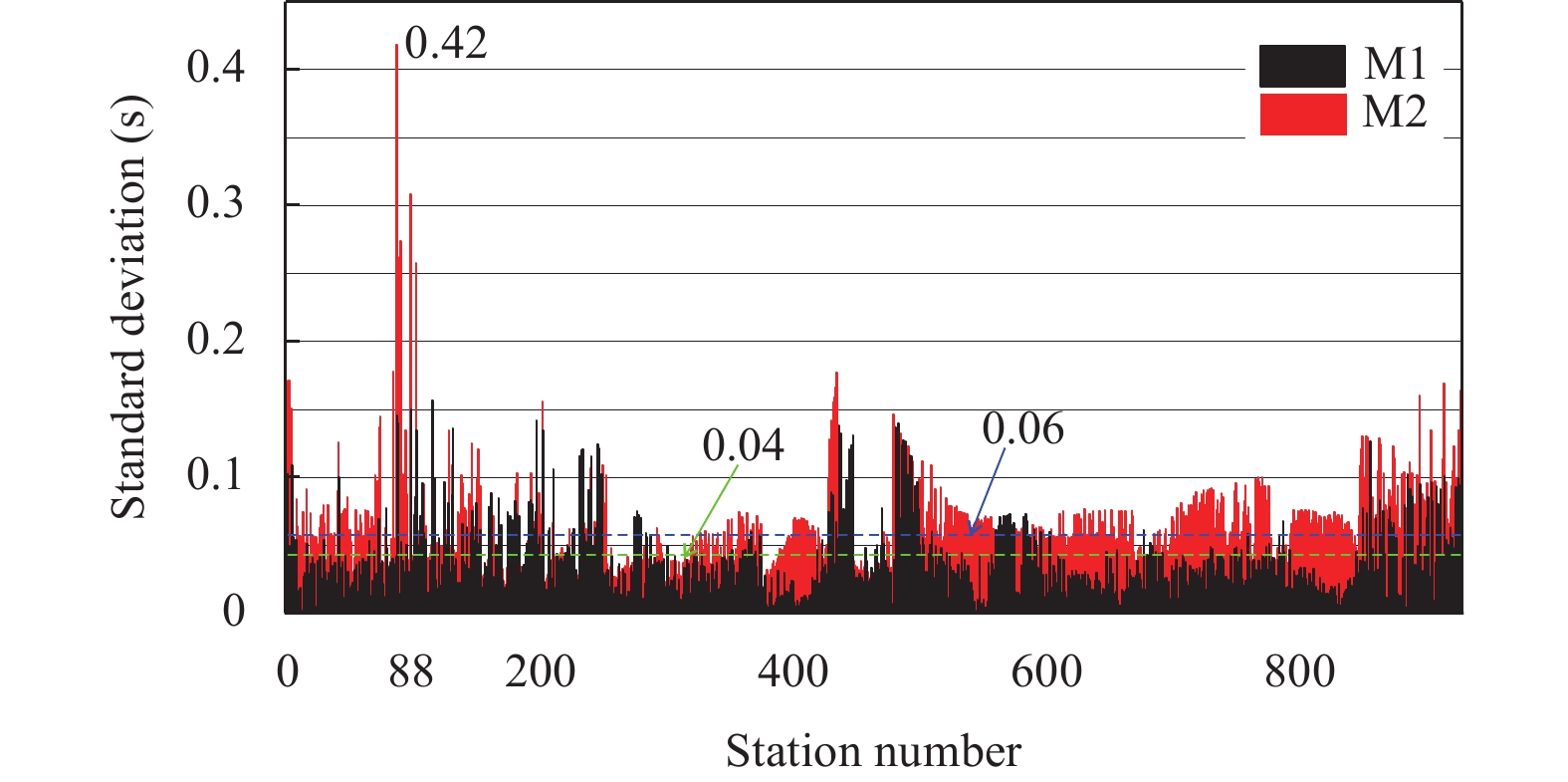
Because the real velocity distribution within the Earth is unknown, we choose four well-known global velocity models, i.e., UU-P07 (Amaru, 2007; Hall and Spakman, 2015), HMSL-P06 (Houser et al., 2008; Tranbant et al., 2012), TX2019slab (Lu C et al., 2019) and GyPSuM (Simmons et al., 2010), to investigate the influences of two measurement methods (M1 and M2). During the investigation of the influences, the heterogeneities inside the target imaging domain can generate extra residual anomalies, which affects the investigation. To eliminate the extra residual anomalies, we build the velocity structure for the NE Tibetan Plateau based on the ak135 reference Earth model (Kennett et al., 1995). Therefore, hybrid models (ak135 layered model inside; global heterogeneous models outside) are constructed for the investigation. Based on these hybrid models, the relative traveltime differences can be calculated by Equations (1) and (3), and are treated as the observed relative traveltime differences. In contrast, the relative traveltime differences are computed based on the ak135, and are regarded as the calculated traveltime differences. Subsequently, we obtain four residuals at each station for each measurement, and the standard deviations of the residuals for M1 and M2 at each station are computed simultaneously. If the standard deviation is zero, the corresponding measurement is not sensitive to the uncertainty in the global model. In contrast, if the standard deviation is large, the measured residual greatly depends on the global model. Therefore, measurements with a small standard deviation are preferred. Note that the M1 measurement depends on the allowed distance for forming station pairs (Liu SL et al., 2018). We choose an allowable distance of 1.5°, which represents the minimal spacing to include all the stations for forming station pairs.

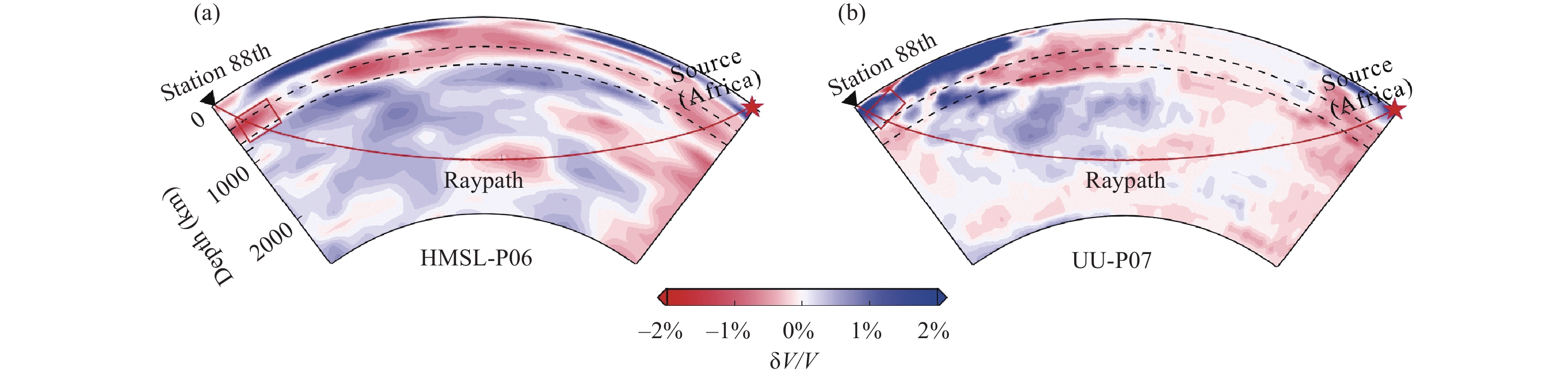
One teleseismic event located at (32.109° E, –7.914° N, 20.0 km) in East Africa and all the stations in the NE Tibetan Plateau are selected to calculate the residuals (Equations 2 and 4). The standard deviations of the residuals at these stations are presented in Figure 2. Evidently, the standard deviations from M1 are generally less than those from M2. The standard deviations from M1 are generally distributed around 0.04 s, while those from M2 are distributed around 0.06 s. In addition, the maximum standard deviation from M2 is 0.42 s, which is about twice as large as that from M1. The large standard deviation is caused by the difference between the velocity models from HMSL-P06 and UU-P07 under the 88th station (96.447° E, 32.196° N, 3.7 km) (Figures 2 and S2). This comparison suggests that the influence of M1 on the measured residuals is smaller than that of M2 if the global reference model employed for the tomographic inversion deviates from the real Earth model.

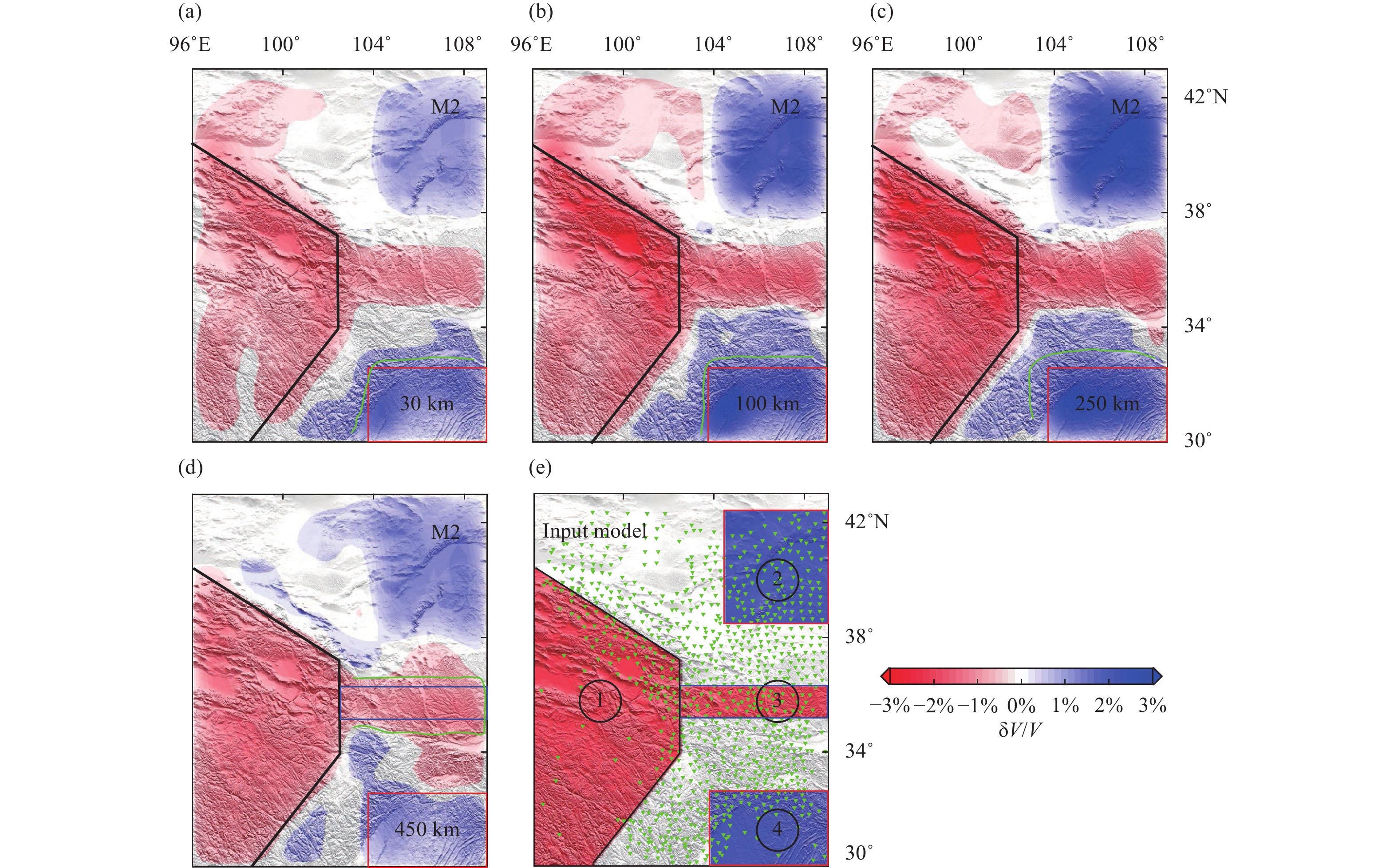
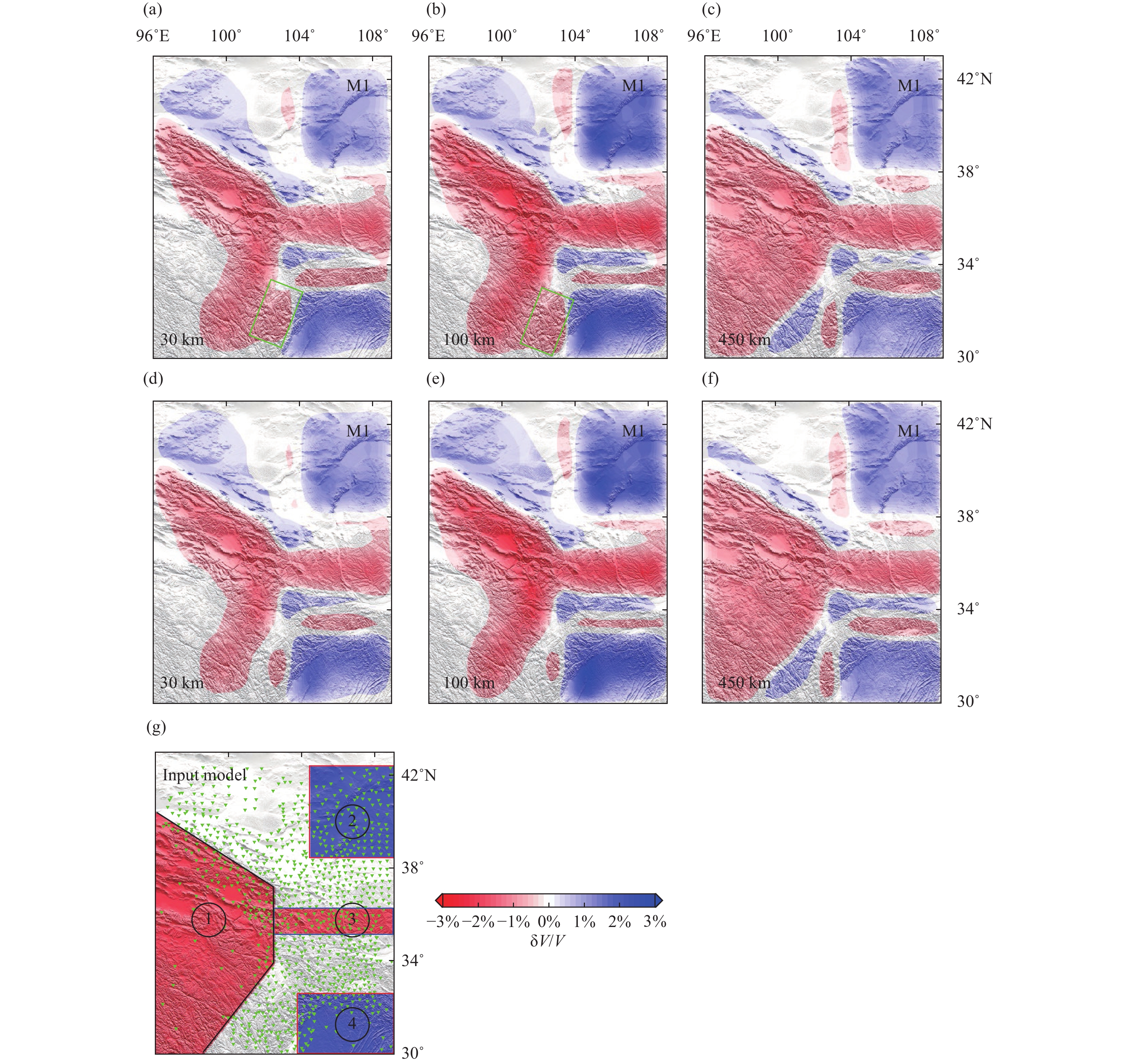
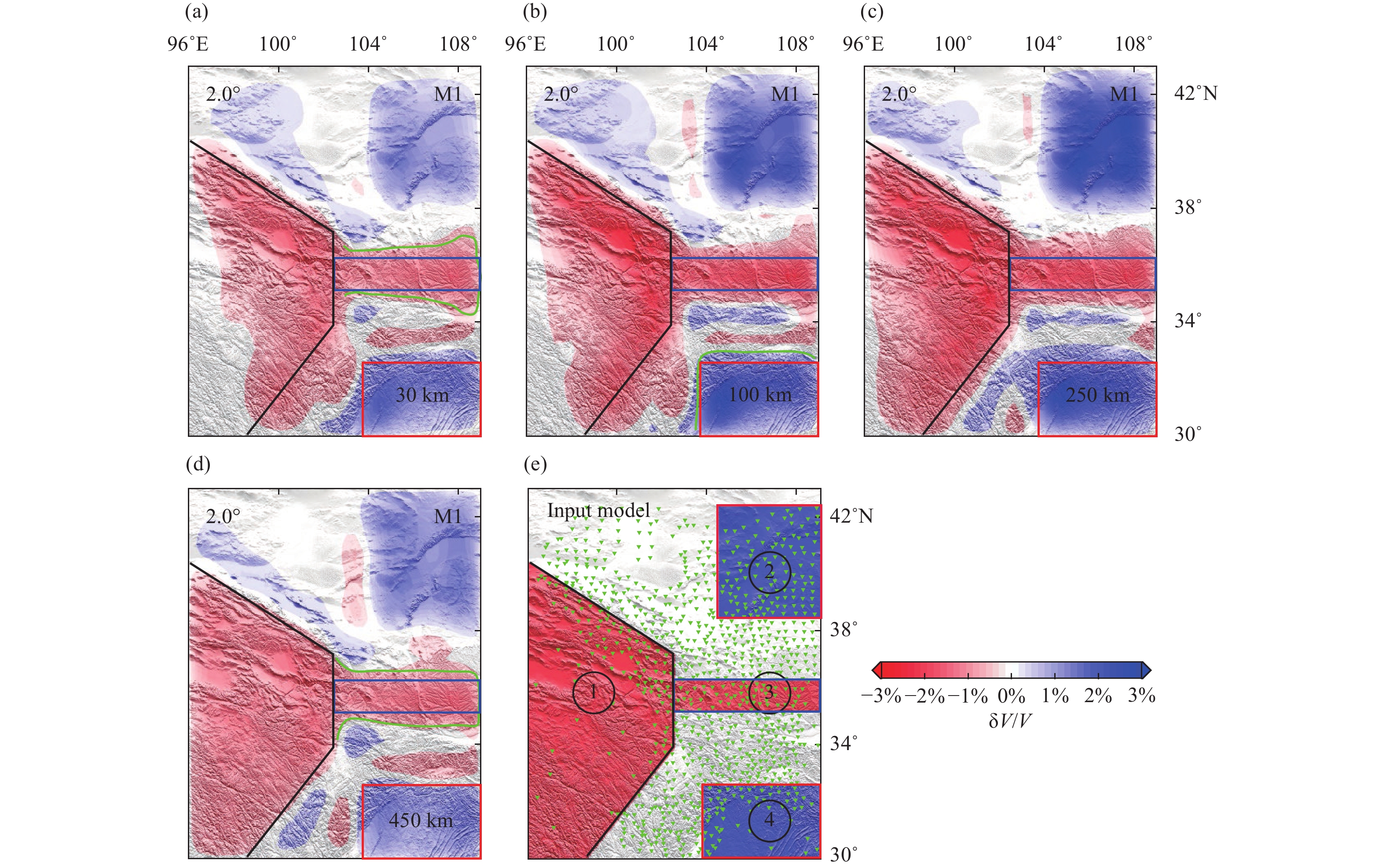
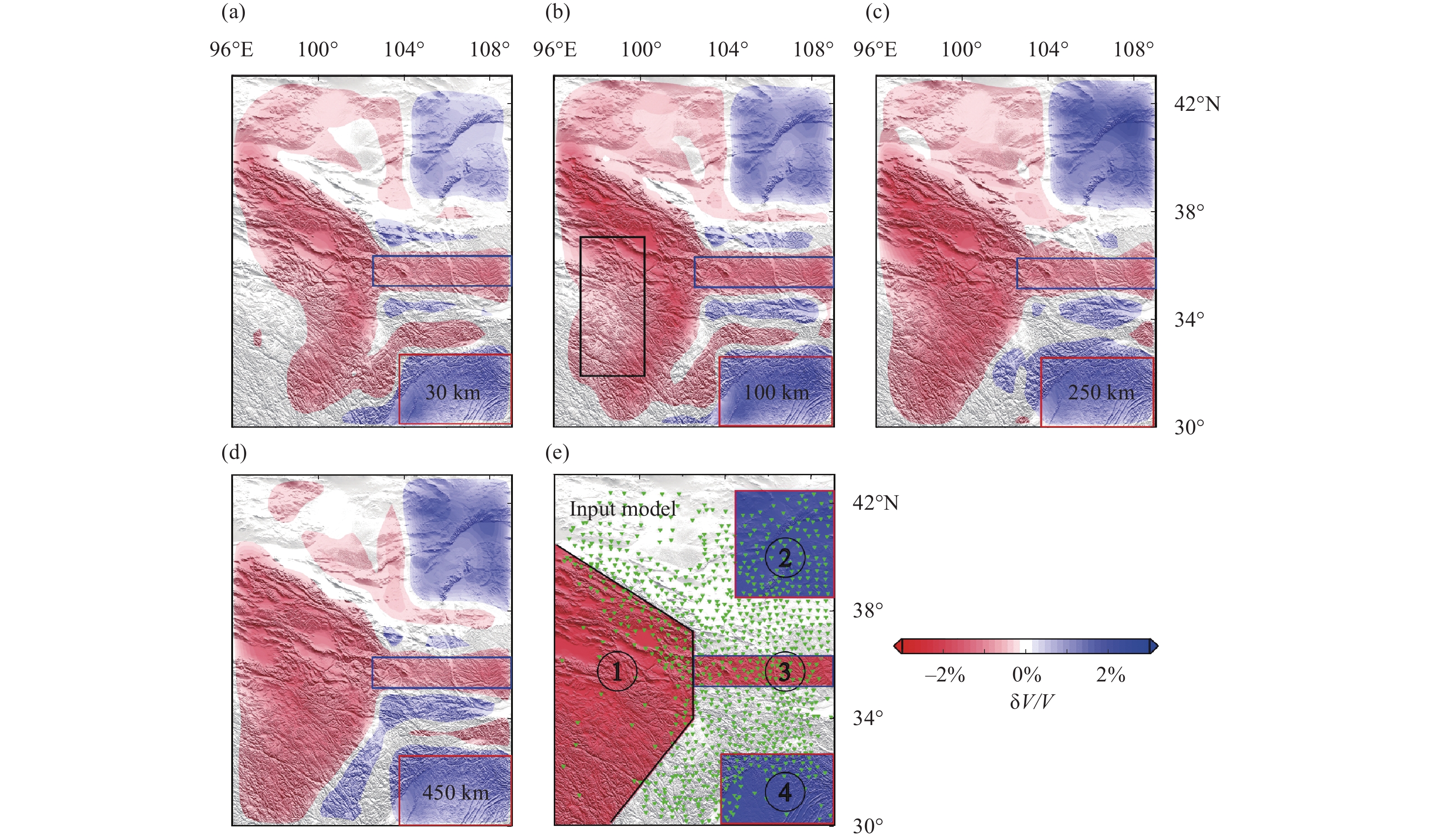
A synthetic tomography test is conducted to further investigate the influences of the measurements. In this test, we treat UU-P07 as the real Earth model. 3-D synthetic structures (Figure 3e) beneath the NE Tibetan Plateau are constructed following the imaging results of Li MY et al. (2022). Then, we select a total of 141 teleseismic events according to the catalog provided by the U.S. Geological Survey (USGS; https://earthquake.usgs.gov/earthquakes/map), and the distribution of these events is shown in Figure 3f. This computation of synthetic data was carried out in the hybrid model consisting of the synthetic structures in the imaging domain and the global model UU-P07 outside. Gaussian noise with a standard deviation of 0.2 s is added to the synthetic data to simulate real data (Lei JS and Zhao DP, 2016; Liu SL et al., 2018). Then we invert the traveltimes in a prior model from the ak135. The inverted images are shown in Figures 3 and 4. Evidently, the number of relative traveltime differences for M1 (Equation 2) is much larger than that for M2 (Equation 4). However, the numbers of the raypaths for M1 and M2 remain the same.

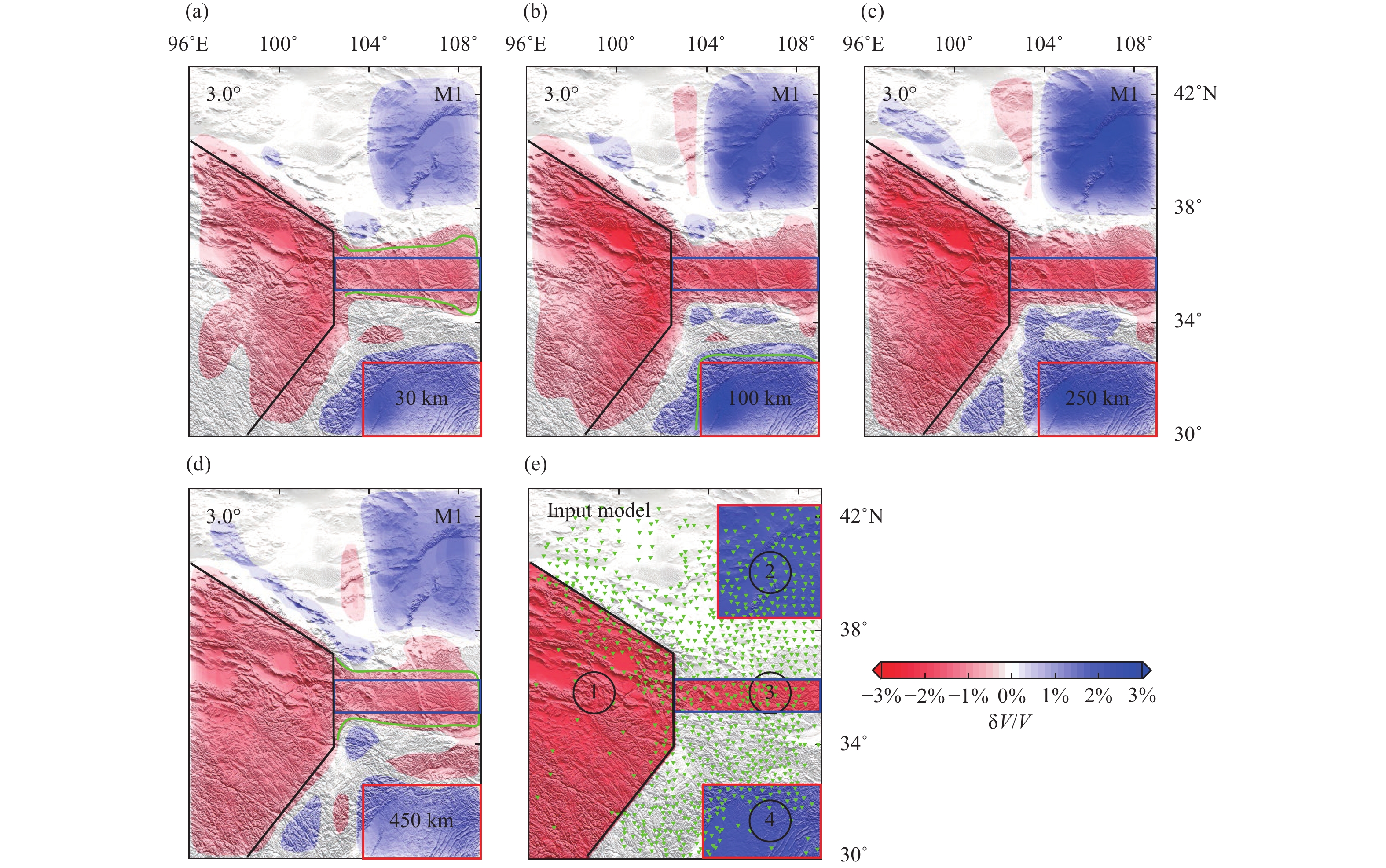
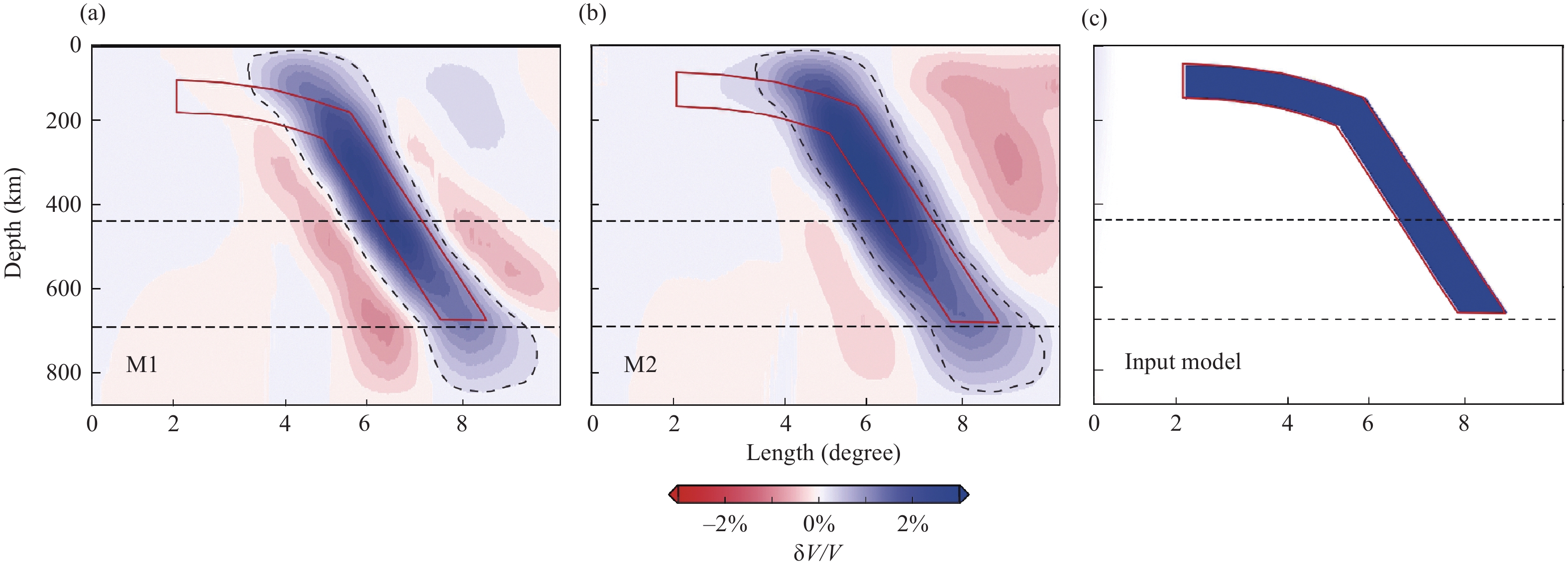
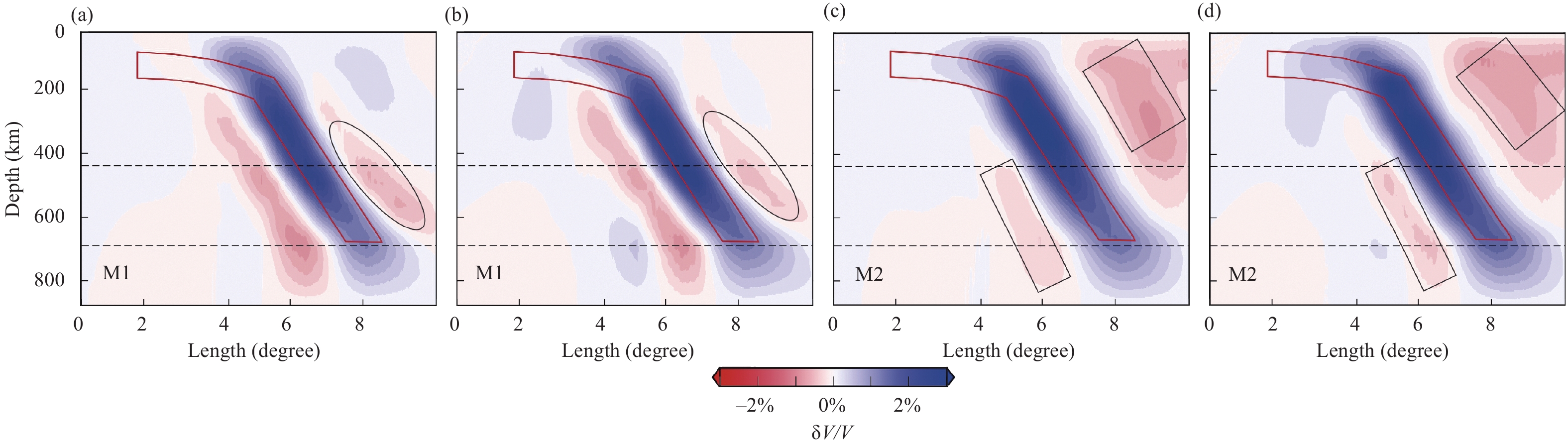
As shown in Figures 3 and 4, the morphology of the synthetic structures is well imaged by both M1 and M2, and the resolution of the imaging results gradually improves from depths of 30 km to 250 km. This increased resolution at depths is because the rays crisscross well at these depths. In addition, we can observe some differences between the images in Figures 3 and 4. First, above 250 km, the large-scale structure (block 1) imaged by M2 is more similar to the input model than that imaged by M1 (Figures 3a–c and 4a–c). Second, the M1 scheme delineates the shape of small-scale structures more clearly (Figure. 3a–d and 4a–d). For instance, block 4 in Figure 3b and block 3 in Figure 3d are well imaged by M1, but the shapes of block 4 in Figure 4b and block 3 in Figure 4d are blurred. Third, the boundary of imaged block 1 is generally sharper in Figure 3a–c than that in Figure 4a–c.

Another test is shown in Figure S3, which inverts a synthetic subduction slab (Figure S3c) below the northern Sumatra (Figure S1a). A total of 26 stations and 1572 events obtained from the USGS are used to compute the ray paths and traveltimes (Figure S1b). The imaging results are presented in Figure S3, which shows that the imaged slab from M1 is sharper than that from M2 at depths greater than 200 km.

4.2   Influence of global mantle heterogeneities

Masson and Trampert (1997) firstly studied the influence of global mantle heterogeneities, and they employed a linear seismic array containing 50 stations with an aperture of 600 km to discuss the influence. In their investigation, they calculated traveltimes from teleseismic sources to their array based on a 1-D layered global reference model and a 3-D heterogeneous global velocity model. Then, for each station, they computed the difference between the two traveltimes calculated from the two global models. They found that the traveltime difference varied considerably across the seismic array, with the maximum difference exceeding 0.2 s. In practical tomography, the relative traveltime residuals employed for the inversion are generally in the domain [−1 s, 1 s] (Rawlinson et al., 2006; Veisi et al., 2021). Thus, the variation in traveltime differences owing to mantle heterogeneities outside the imaging domain has nearly the same order of magnitude as the relative traveltime residuals observed by the seismic array. Therefore, it is reasonable to speculate that global mantle heterogeneities may impact the imaging results because of the large variation in traveltime differences. This speculation was demonstrated by a tomographic inversion with real data in Lei JS and Zhao DP (2016), who introduced a heterogeneous global velocity model (Lei JS and Zhao DP, 2006) to calculate the traveltimes of teleseismic earthquakes, and obtained a tomographic model for eastern Tibet. Accordingly, they reported some detailed structures and found that the amplitudes of the velocity anomalies changed slightly. As noted by Zhao DP et al. (2013), the data coverage determines the first-order features of tomography images. For typical teleseismic tomography, the data coverage is generally sufficient. Therefore, the first-order features are unlikely to be changed due to the influence of global mantle heterogeneities (Lei JS and Zhao DP, 2016).

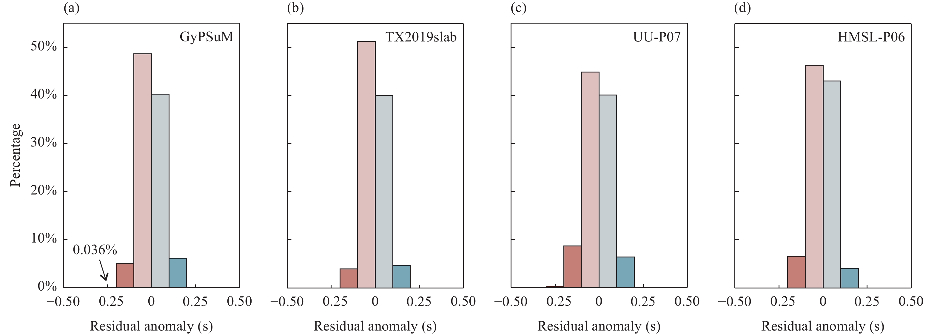
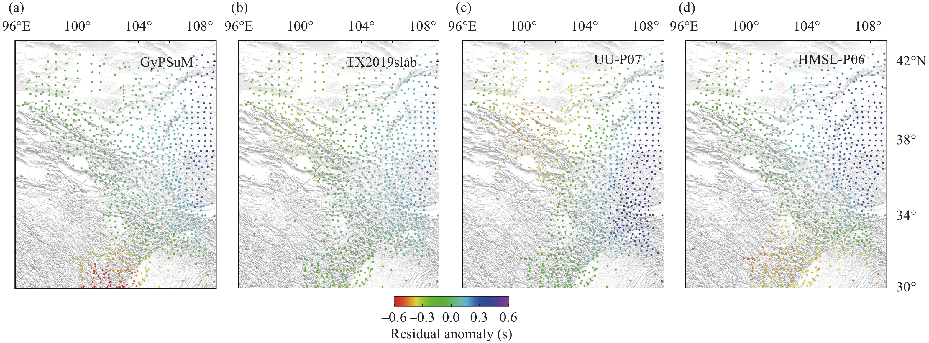
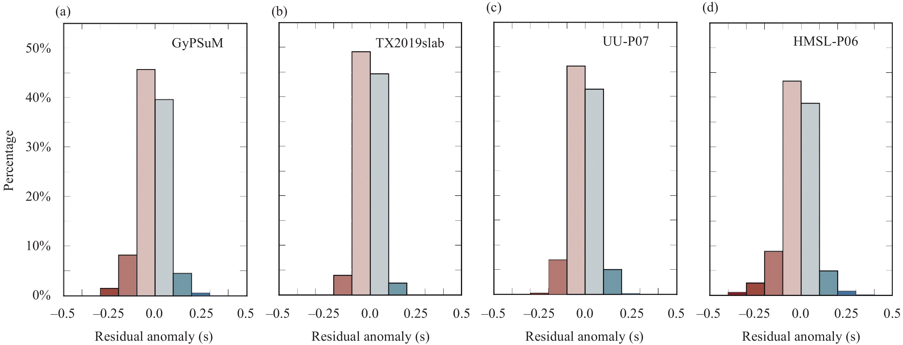
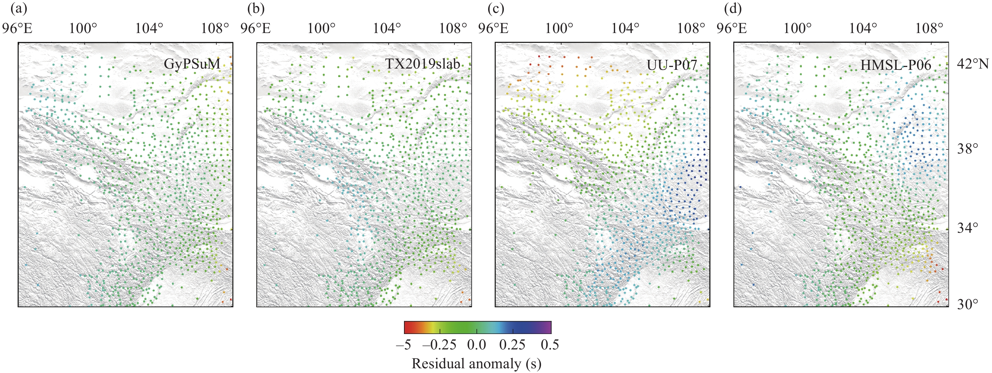
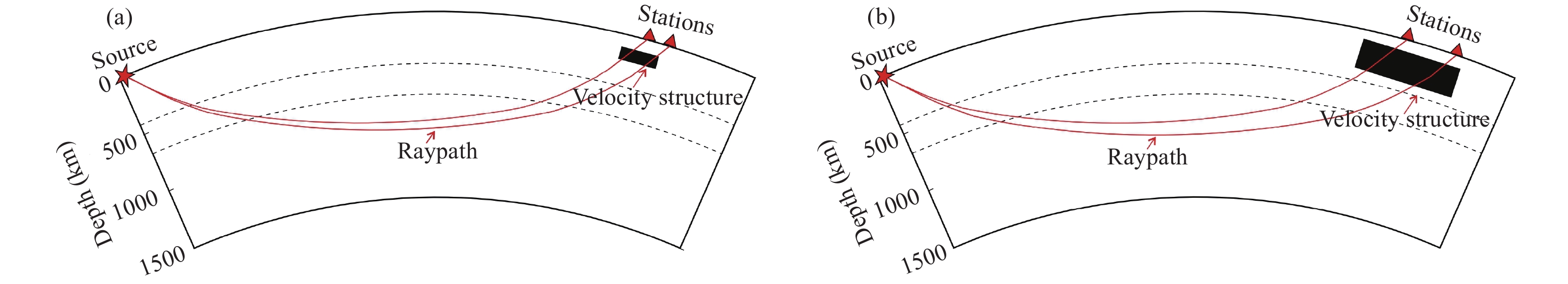
Following Masson and Trampert (1997) and Zhao DP et al. (2013), we employ the four global models presented in the above subsection to further study the influence of global mantle heterogeneities. We adopt three steps to exactly calculate the anomalies of the residuals owing to mantle heterogeneities and exclude the influence from the heterogeneities inside the imaging domain. First, we calculate seismic rays from a source to the stations in each global model. Second, stations on the surface (Figure 1) are projected to the cross points, where the seismic rays pass through the bottom of the target volume. Third, the stations on the cross points are treated as virtual stations, and relative traveltime differences are computed based on the virtual stations. To sample complex structures within the Earth, we choose three teleseismic events with different epicentral distances and azimuths. The first event occurred in East Africa at coordinates of (32.109° E, –7.914° N, 20.0 km); the rays from this event are expected to sample the African superplume (Ni SD et al., 2002; Park and Nyblade, 2006). The second event is located at (154.524° E, 46.243° N, 10.0 km) near the southern end of the Kuril Trench (Wang ZW and Zhao DP, 2021); the seismic rays from this event should pass through the subducted Pacific lithosphere (Chen M et al., 2015). The third event is the M_W9.3 Indian ocean earthquake in Sumatra with a hypocenter of (95.982° E, 3.295° S, 30.0 km) (Stein and Okal, 2007; Subarya et al., 2006); the seismic rays from this event sample the complex velocity structure of the Andaman-Sumatra subduction zone (Hall and Spakman, 2015; Wang X et al., 2022). On the basis of these sources and virtual stations, we calculate the residual anomalies in four global models by using M1 and M2. The results are shown in Figures 5–6, S4–S5, and S6–S7.

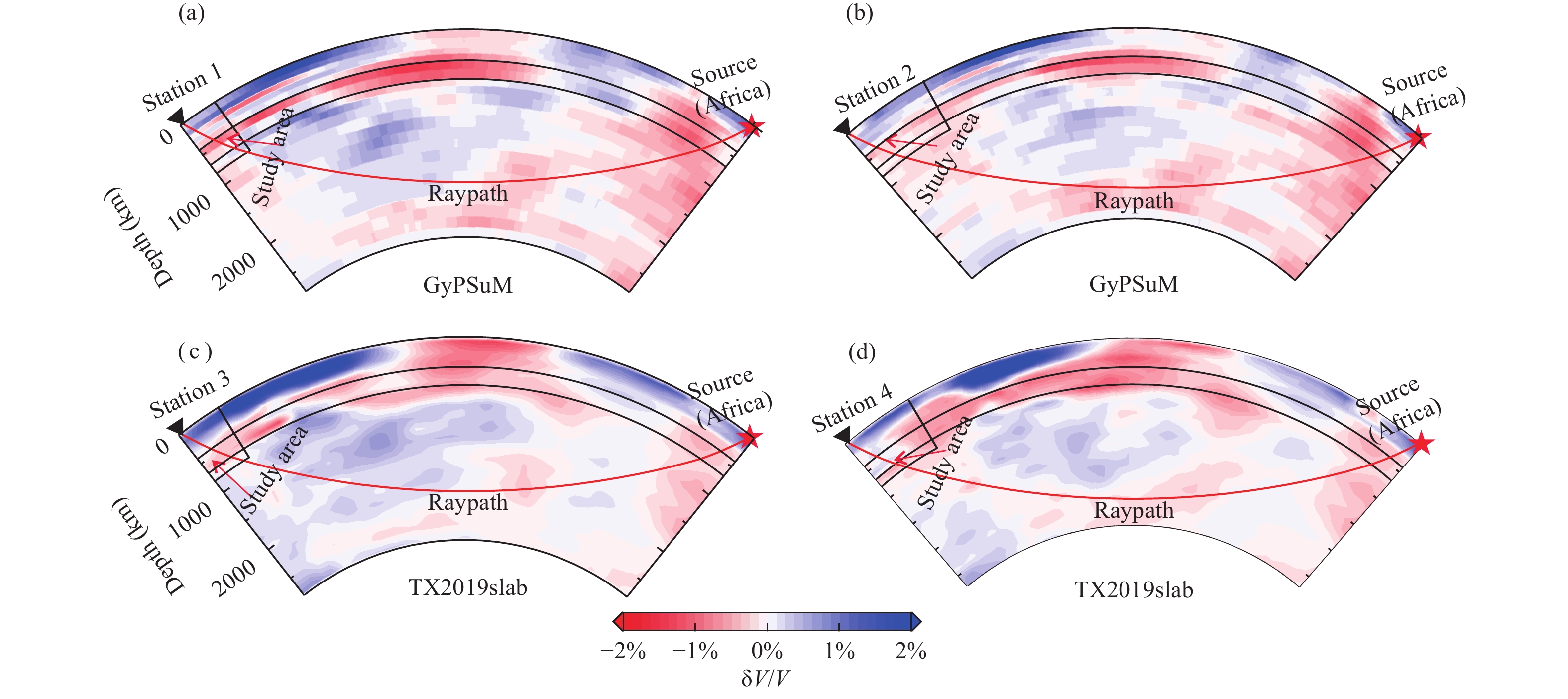
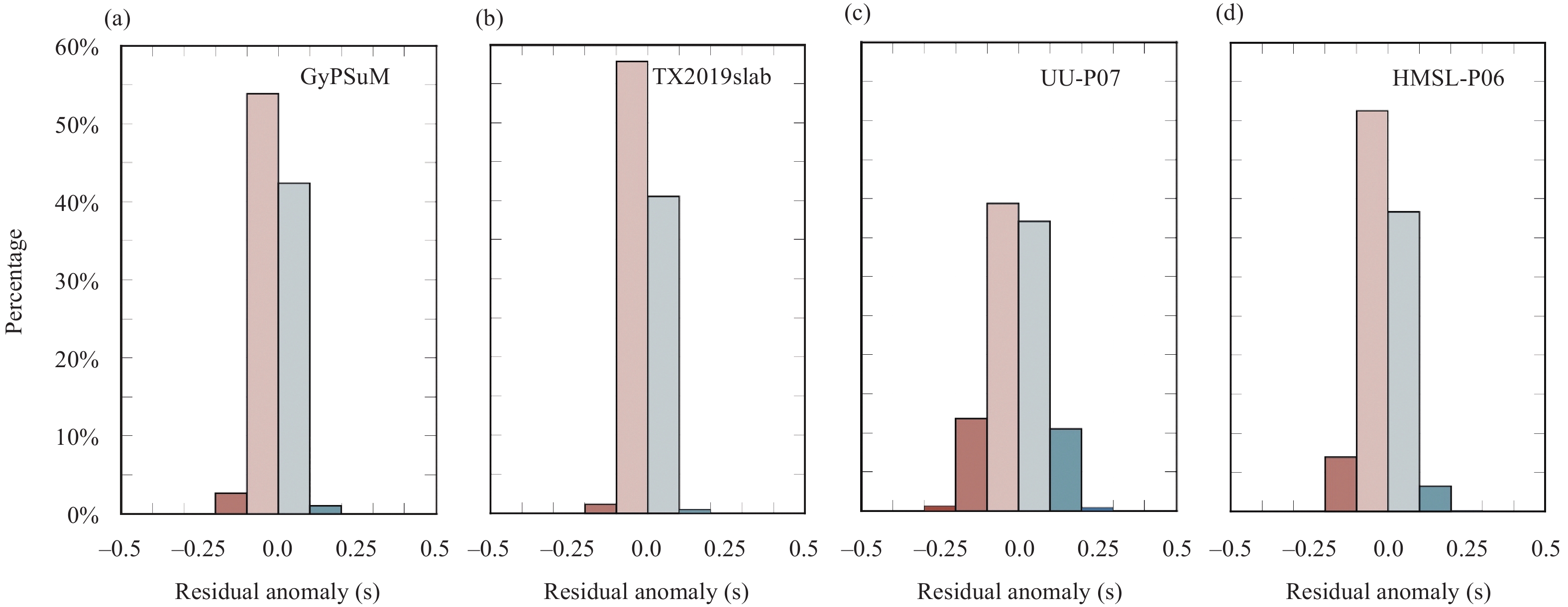
Figures 5 and 6 show the residual anomalies for the teleseismic event in East Africa. The residual anomalies generally vary from about −0.6 s to 0.6 s. For M1, the maximum residual anomaly is −0.28 s, which appears when we choose GyPSuM ( Figure 5a). For the same global model, the residual anomalies calculated from M2 are also large (Figure 6a), and the maximum value is −0.55 s. The significant negative residual anomalies in GyPSuM ( Figure 6a, such as at Station 1) are caused by the rays sampling a strong high-velocity near the study area (Figure 7a). In contrast, the remarkable positive residual anomalies in GyPSuM (Figure 6a, such as Station 2) are mainly due to the low-velocity structures in the lower mantle under the India Plate (Figure 7b). Similarly, the prominent residual anomalies at Station 3 and Station 4 can also be explained by station-side mantle heterogeneities. It is noteworthy that residual anomalies for different sources in the same global model vary greatly (Figures 5–6, S4–S5 and S6–S7). This variation in residual anomalies is due to the rays sampling different structures of the global model.

Synthetic tests are conducted to study the influence of global mantle heterogeneities on tomographic images. In these tests, we select UU-P07 to generate the residual anomalies, which incorporate the influence of global mantle heterogeneities. Gaussian noise with a standard deviation of 0.2 s is added to synthetic data to mimic the random noise in real data. The tomography results using the M1 (the allowable distance of 1.5°) are shown in Figure 8a–c. For the purpose of comparison, we also present the tomography results without the influence of global mantle heterogeneities (Figure 8d–f). From the comparison, we find that the main image pattern is not changed by the influence of global mantle heterogeneities (Figure 8). However, some artifacts appear in Figure 8a and 8b (green rectangle). We find similar results by another synthetic test using M2 (Figure 9).

We also present the inversion results of the subducted slab with and without the influence of mantle heterogeneities in Figure S8. The mantle heterogeneities do not affect the morphology and amplitude of the subducted slab in the inversion results. However, the amplitude of the artifacts varies due to the global mantle heterogeneities (Figure S8a and S8b; Figure S8c and S8d).

4.3   Influence of the station spacing

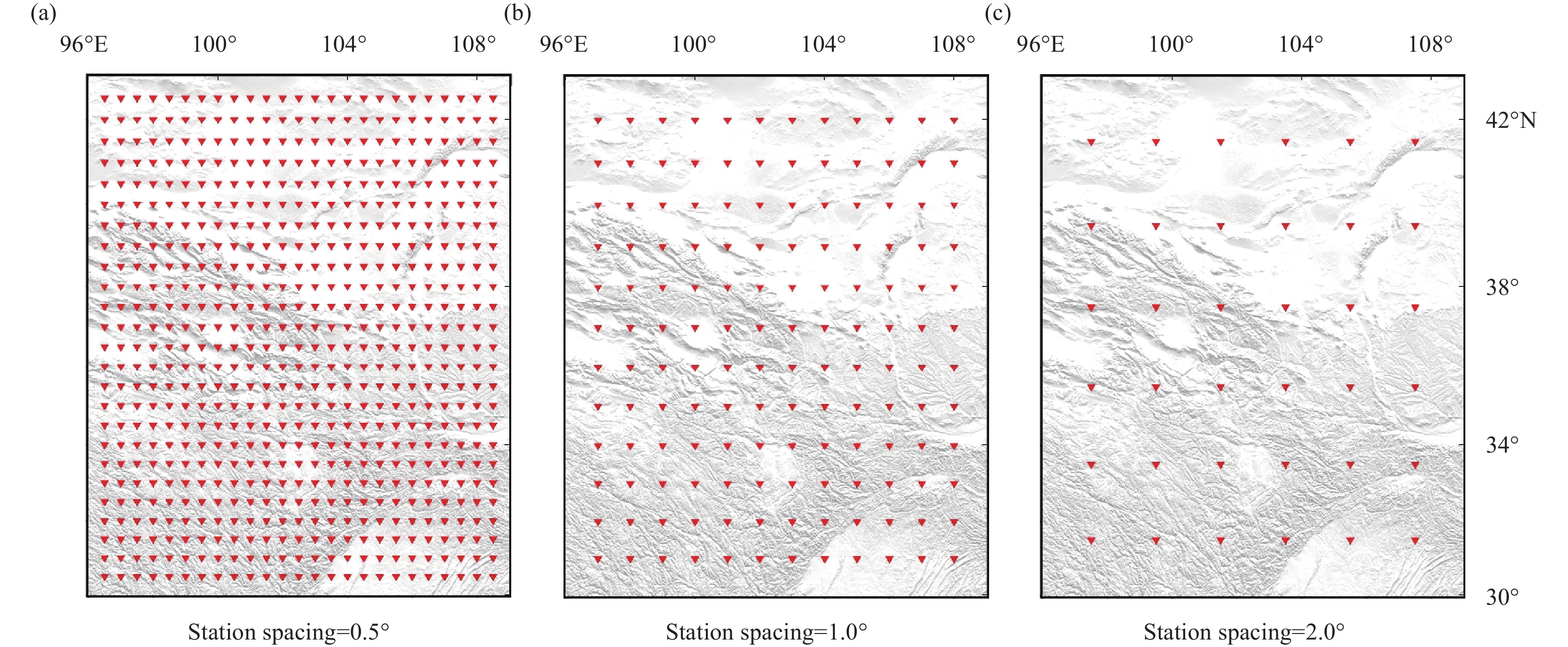
Liu SL et al. (2018) pointed out that station spacing affects the imaging accuracy of teleseismic traveltime tomography when using M1. A large station spacing may introduce imaging artifacts owing to mantle heterogeneities. To eliminate imaging artifacts, the distance between two adjacent stations for measuring the relative traveltime difference must be sufficiently small (Liu SL et al., 2018; Li MY et al., 2022). However, it is difficult to define the threshold for such a sufficiently small distance in practical teleseismic tomography. In typical teleseismic tomographic studies, the minimal station spacing may range from 0.05º to 3.0º (Steck et al., 1998; Rawlinson et al., 2006; Liu SL et al., 2018, 2019, 2021; Bai T et al., 2020; Yao JY et al., 2021; Li MY et al., 2022). However, if only station pairs with interstation distances close to the minimal station spacing are involved in the tomographic inversion, the number of seismic rays may not be adequate, in which case the tomographic accuracy cannot be guaranteed. Generally, a distance greater than the minimal spacing distance is adopted to form station pairs. Evidently, the allowed distance for forming station pairs and the number of rays involved in tomographic inversion exhibit a trade-off. To determine the optimal allowed distance, Liu SL et al. (2018) proposed an L-curve method that is able to balance this trade-off. The L-curve method is used by Li MY et al. (2022) to determine the optimal allowed station spacing in the tomography study of northeastern Tibetan Plateau. However, the imaging accuracy is not explicitly taken into account, and the influences of source uncertainties and global mantle heterogeneities under the condition of this allowed distance have not yet been quantitatively evaluated.

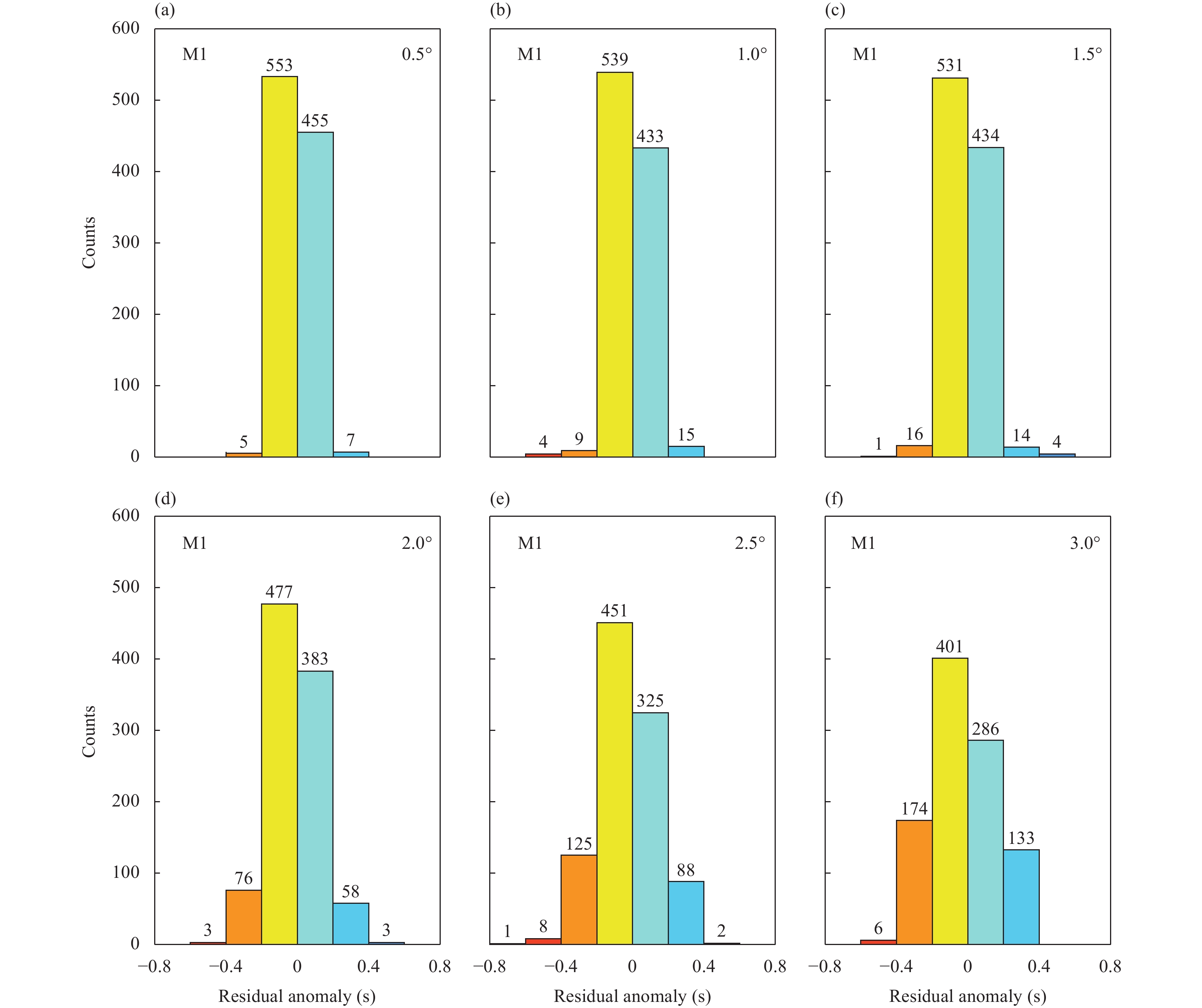
To further investigate the influence of the station spacing on M1, we employ the teleseismic events in East Africa and the 927 stations to compute the traveltimes in a hybrid model. We embed the synthetic structures in the target volume (Figure 3f) into two global models, ak135 and UU-P07, to construct two hybrid models. The one with the ak135 is denoted Model 0; while the other is named Model 1. The traveltimes computed in Model 0 and Model 1 are treated as calculated and observed traveltimes, respectively. For a given distance to form station pairs, we can calculate the relative traveltime residuals based on Equation (2). For different given distances, we obtain different sets of residuals. We plot the sets of residuals with distances of 0.5°, 1.0°, 1.5°, 2.0°, 2.5° and 3.0° in Figure 10a–f, respectively. Note that the station spacing represents the average distance for forming station pairs. The distances for station pairs are in a certain range, which is presented in Table S1.

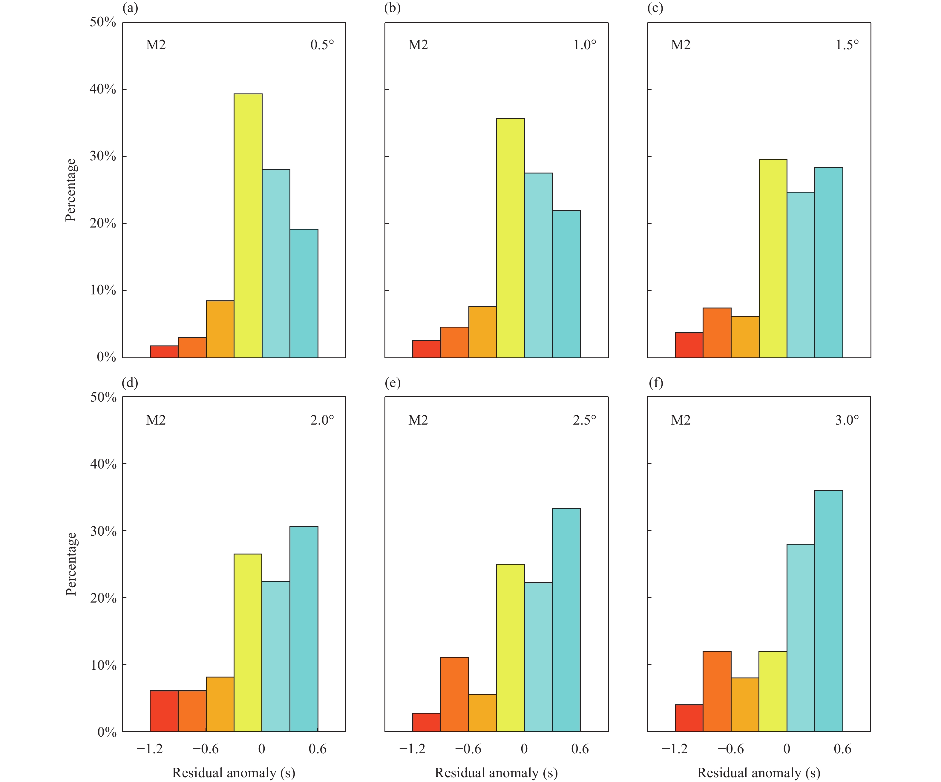
For the fixed distribution of stations in Figure 1, it is difficult to investigate the influence of station spacing for M2. To resolve this difficulty, we have to construct several station arrays with average station spacings of 0.5°, 1.0°, 1.5°, 2.0°, 2.5° and 3.0° around the center of the study area (Figure S9). The residuals for M2 with different average station spacings are shown in Figure 11. For M1, the number of residuals with large values (> 0.2 s) generally increases with the station spacing (Figure 10), while for M2, the number of residuals with large values (> 0.2 s) slightly increases with the station spacing (Figure 11).

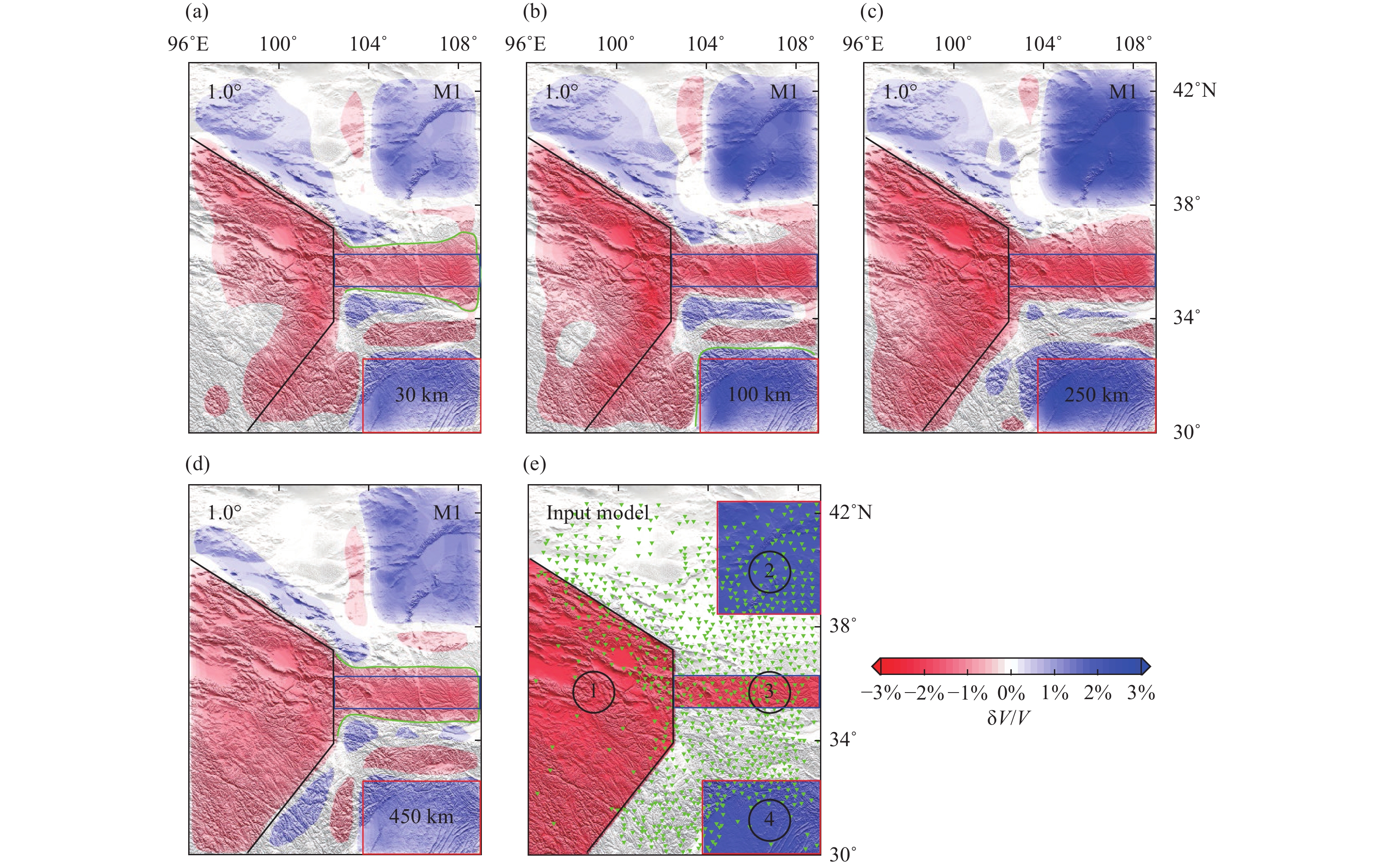
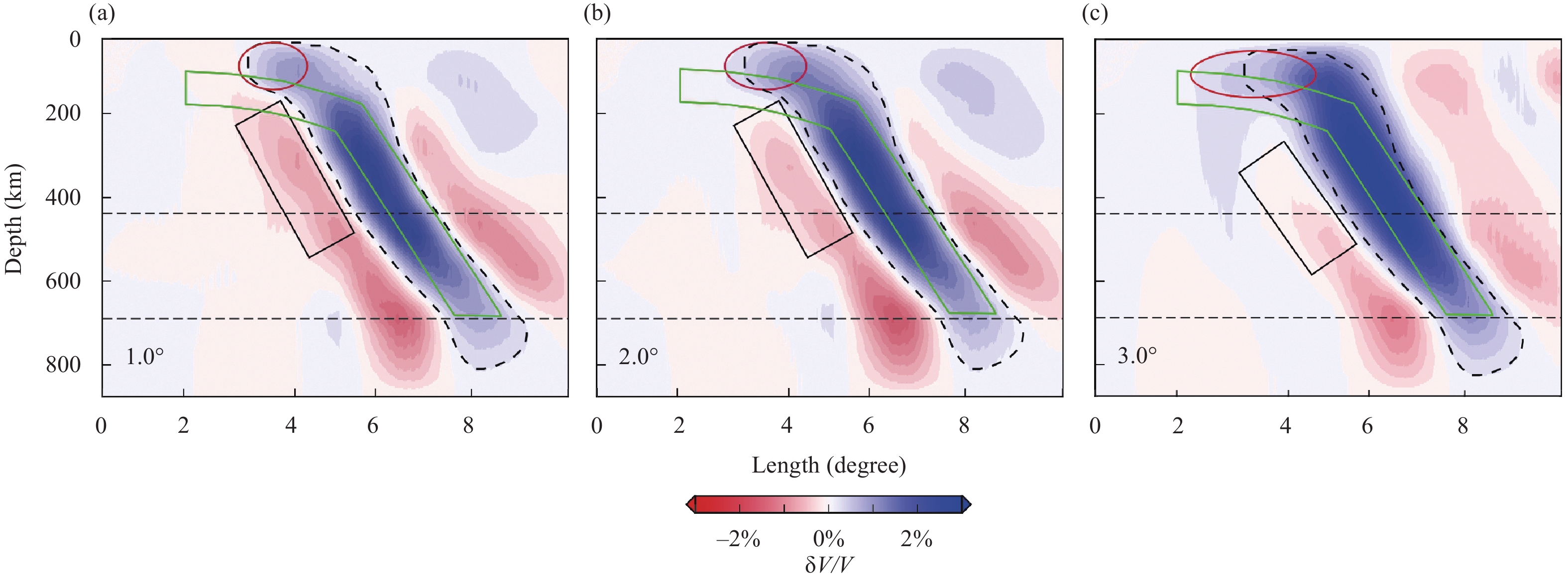
We conduct synthetic tomography tests to further investigate the influence of the station spacing. Because similar results and conclusions may be obtained by using M2, we only choose M1 for the discussion of station spacing. The inversion results with station spacings of 1.0°, 2.0° and 3.0° are shown in Figures 12–14, respectively. From these figures, we can observe two features. First, above a depth of 100 km, the images of long wavelength structures (such as block 1) gradually improve with increasing station spacing (Figures 12a, 12b, 13a, 13b, 14a and 14b). Second, the width of imaged block 3 slightly increases with station spacing (Figures 12d, 13d and 14d).

We also image the subducted slab in northern Sumatra using station pairs with different station spacings. It should be noted that the minimum distance to include all the stations (Figure S1a) to form station pairs is about 2.5°. Therefore, we add some fictitious stations (19 stations) to increase the density of the seismic network in northern Sumatra, which facilitates the setting of different distances for forming station pairs in the tomographic inversion with M1. The images from the synthetic tomography tests are displayed in Figure S10, which are obtained by using station pairs with station spacings of 1.0°, 2.0° and 3.0°. As shown in Figure S10, the main feature is that the width of the imaged slab increases with the station spacing. In addition, the scale of the low-velocity anomaly below the imaged slab decreases with increasing station spacing (black rectangles in Figure 10); this phenomenon is attributed to the station distribution. Although 19 fictitious stations are added for the synthetic tests, the stations (Figure S1a) are still distributed along the mainland of Sumatra, meaning that the station density is sparse in the NE-SW direction. Thus, when the station spacing is 1.0°, few station pairs oriented NE-SW are included in the tomographic inversion. As the station spacing increases, however, more station pairs oriented NE-SW are included. Therefore, the tomography tests show a tendency to resolve the horizontal portion of the synthetic slab at shallow depths (red ellipsoid in Figure S10) and reduce the low-velocity artifact below the imaged slab.

4.4   Influence of source uncertainties

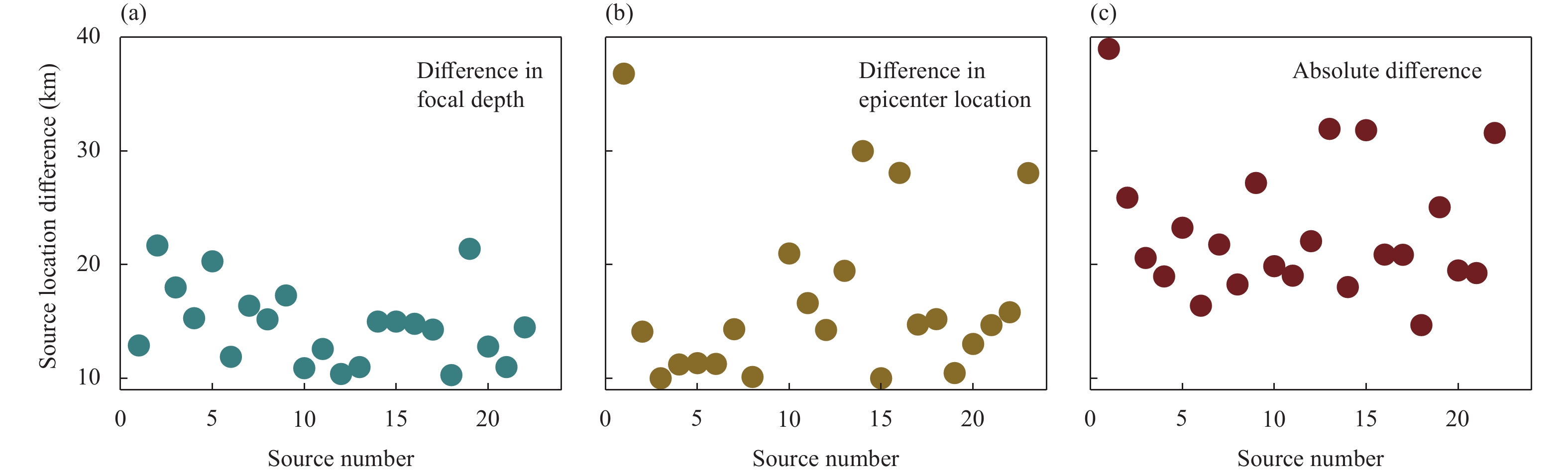
Aki et al. (1977), Zhao DP et al. (1994), Lippitsch (2003) and Rawlinson et al. (2006) indicated that the relative traveltime difference can minimize the effect of source uncertainties. However, direct evidence is absent. Therefore, we conduct synthetic tests to provide direct evidence. According to the two catalogs provided by the International Seismological Centre (ISC; http://www.isc.ac.uk/) and the USGS, we obtain 1003 teleseismic events from 2018 to 2020. The hypocenter differences between the two catalogs are simply considered as source uncertainties. By comparing the two catalogs, we retain the events with uncertainties of the focal depths and epicenter locations greater than 10 km. Eventually, we select a total of 22 events. The uncertainties of depth, epicenter and absolute location are shown in Figure 15a–c, respectively. As shown in Figure 15, the uncertainties are very large. The uncertainties of the hypocenters are about 25 km. The maximum perturbation of focal depth is about 22 km (Figure 15a).

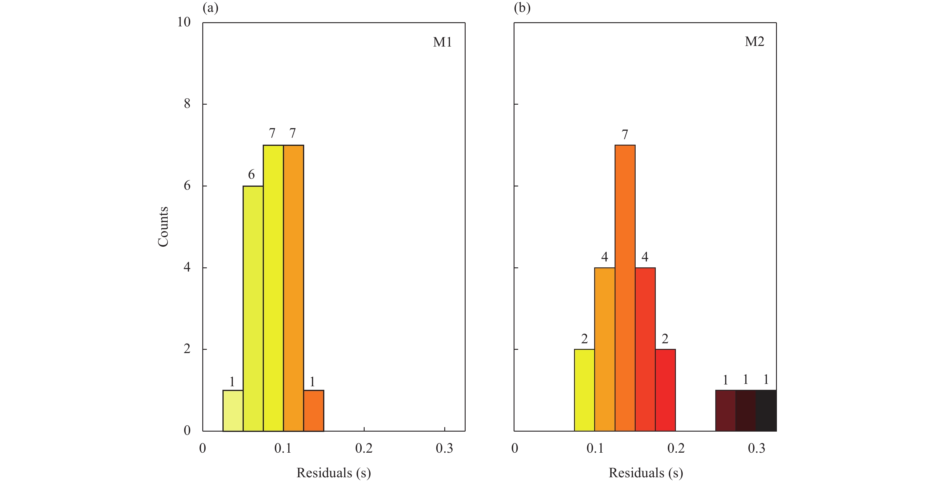
The influence of source uncertainties for each measurement can be measured in two steps. First, the two sets of hypocenter locations provided by ISC and USGS are employed to calculate traveltimes in a global model (UU-P07), and we simultaneously compute the relative traveltime differences. Note that station spacing of 1.5° is used for M1. Second, the influence of source uncertainties is measured by calculating the values between the two sets of relative traveltime differences. For visualization purposes, we select the maximum absolute value among all stations for each earthquake and display the value in Figure 16.

As shown in Figure 16, the values from M1 for evaluating the influence are generally less than 0.1 s; while the values from M2 are generally less than 0.2 s. Evidently, residual anomalies caused by source uncertainties are much smaller than those from mantle heterogeneities (Figures 5 and 6). Sources with uncertainties of about 25 km do not produce significant anomalies. Actually, sources with uncertainties of about 25 km are actually rare in practice (Pesicek et al., 2010). Therefore, we consider that the source uncertainties are probably not able to generate evident imaging artifacts, and we do not conduct any further synthetic tomography tests for this influence.

5.   Discussion

Although previous studies discussed some aspects of influencing factors on teleseismic tomography (Aki et al., 1977; Masson and Trampert, 1997; Rawlinson et al., 2006; Foulger et al., 2013; Zhao DP et al., 2013; Lei JS and Zhao DP, 2016; Liu SL et al., 2018), comprehensive analysis is necessary. Based on extensive synthetic tests, we discuss the influencing factors.

In the same global heterogeneous model, the influence from M1 is smaller than that from M2. With the accumulation of seismic data (Sambridge and Faletič, 2003; Simmons et al., 2012; Lu C et al., 2019) and the employment of different techniques (Bijwaard et al., 1998; Obayashi et al., 2013; Lei WJ et al., 2020) for global tomography, updated global models are able to interpret an increasing number of observations. Although the global models can effectively approximate the Earth, they are not an actual Earth model. Therefore, model uncertainties are inevitable among the existing global models. In Figure 2, the standard deviation for M1 is smaller than that for M2. The smaller standard deviation indicates that the influence from the real Earth model for M1 is probably less than that for M2. Evidently, the two raypaths for a station pair in M1 are generally closer to each other than those in M2 (Equations 2 and 4). Therefore, the raypaths for a station pair in M1 are more likely to sample the same structures even if the real Earth has small-scale structures. Thus, M1 is less sensitive to the uncertainty in the global model.

Based on the synthetic tomography test (Figures 3 and 4), we can conclude that the model is well imaged by both the M1 and M2, and the imaging results are generally similar. However M2 has an advantage in imaging long wavelength structures. While the resolution of M1 is slightly higher than that of M2 (Figures 3, 4 and S3), the ability of M1 to image long wavelength structures is reduced. We can explain this phenomenon based on Equations (1)–(4). For M1, each residual calculated for a station pair is sensitive to the structures sampled along the seismic ray paths recorded at both stations. The distance between the two seismic rays for each station pair is proportional to the spacing of the station pair. Therefore, a small station spacing may better detect fine subsurface structures, and a large spacing is better to image large-scale structures. Given a constant number of station pairs, a higher resolution can be achieved from M1 with a smaller station spacing, as is demonstrated by Figures 3 and S3. Specifically, the definition of M2 in Equation (4) is similar to that of M1 in Equation (1). We can rewrite Equation (4) as

Compared with the definition of Equation (2), Equation (4) includes not only the station pairs with small spacings but also the station pairs with large spacing (the maximum distance is equal to that between the two stations with the greatest spacing). Owing to the inclusion of station pairs with large spacings, M2 can better image the large-scale structures, but the tomographic resolution with M2 is reduced relative to that with M1. This phenomenon of different station spacings being sensitive to different structure scales is evident in Figures 12-14 and S10. With the increasing in station spacing, the image of large-scale structures is improved, however the resolution slightly decreases (Figures S10 and S11).

For M1 and M2, it is difficult to conclude that one is better than the other. In practical teleseismic traveltime tomography, an optional strategy to obtain better tomographic results is to combine M1 and M2, which forms a two-step inversion method. First, the general velocity structures can be inverted by the M2. Second, the inverted velocity structures can be treated as the initial model for the inversion by the M1. In the two-step inversion, the inversion parameters for each inversion are different. Specifically, the damping parameters in the second step are generally smaller than those in the first step, which may lead to similar results as those from one-step inversion with M1.

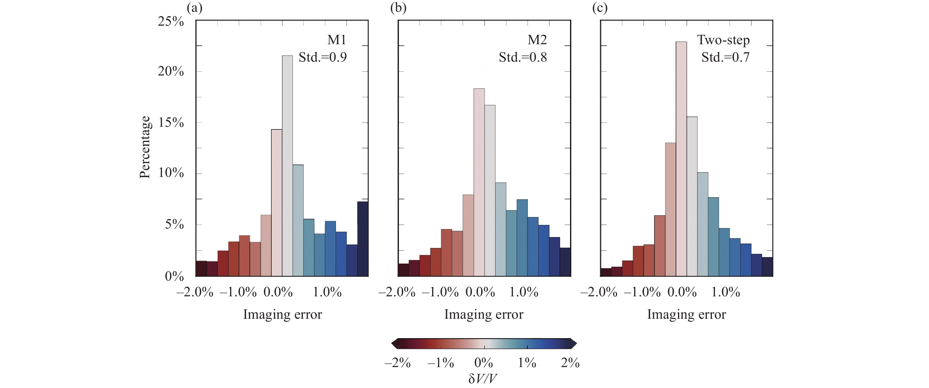
Figure 17 show the tomographic images of the NE Tibetan Plateau after the two-step inversion. The two-step inversion not only provides long wavelength structures, but also delineates the shape of structures with high accuracy. Comparing the results from the two-step inversion (Figure 17) with those from one-step inversion (M1 or M2) (Figures 3 and 4), the two-step inversion is generally better than one-step inversion. A quantitative comparison is presented in Figure S12, which presents the standard deviations of imaging errors from one- and two-step inversions. Clearly, the two-step inversion achieves the smallest imaging errors. Note that the two-step inversion may introduce additional artifacts compared with one-step inversion. However, the artificial features are not emphasized (Figures 3, 4 and 17). Besides, other inversion method may also combine the advantages of M1 and M2 similar to the two-step inversion method. For example, the relative traveltime differences measured by M1 and M2 can be inverted simultaneously. The results from the joint inversion are shown in Figure S14. The joint inversion combines the advantageous of M1 and M2 (such as the ability of recovering long wavelength structure and sensitivity to fine structure).

In this article, we only focus on linear inversion, and a rule of thumb for the distance of the station pair can be obtained from our synthetic tests. For example, the imaging resolution of both the NE Tibetan Plateau and northern Sumatra is about 1° and it is 3° for the maximum distance for forming station pairs to achieve high imaging resolution. Therefore, the maximum distance for M1 is suggested to be three times as the scale of the imaging resolution. Accordingly, the minimum distance for M1 is suggested to be no less than the scale of the imaging resolution to image the long wavelength structures.

Because of global mantle heterogeneities, the calculated residuals (Equations 2 and 4) contain the residual anomalies resulting from mantle heterogeneities outside the imaging domain. In traditional tomography, a layered global model, such as the ak135 or iasp91 (Kennett and Engdahl, 1991), is employed to approximate the velocity structures outside the target imaging domain (Zhao DP et al., 1994; Liu SL et al., 2018), which are not inverted simultaneously with the velocity structures inside the imaging domain. Therefore, the residual anomalies originating from external mantle heterogeneities are partially projected onto the velocity anomalies inside the imaging domain, which generates artifacts (Figure 8a and 8b; Figure 9a–c; Figure S8a and S8c). The mapping of residual anomalies into the imaging structures is also pointed out by Foulger et al. (2013). Nevertheless, although the influence of mantle heterogeneities introduces imaging artifacts, the amplitudes of these artifacts are much weaker than those of the target image (Figures 8, 9, S8a and S8c). The azimuthal coverage of teleseismic events is generally good (Figures 3f and S1b), and most seismic rays probably do not sample a common velocity anomaly. Therefore, coherent residual anomalies are unlikely to be generated. Thus, although the maximum residual anomaly can reach 0.55, significantly strong artifacts do not appear in the tomographic images (Figures 8, 9, S8a and S8c). To obtain tomographic images with greater accuracy, it is necessary to take global mantle heterogeneities into account. With the accumulation of seismic data (Sambridge and Faletič, 2003; Simmons et al., 2012; Lu C et al., 2019) and the development of imaging techniques (Bijwaard et al., 1998; Obayashi et al., 2013; Lei WJ et al., 2020), the global tomographic models are more and more accurate, which creates the benefit for mantle correction in the future.

According to our study, the residual anomalies caused by source uncertainties are not enough to produce evident effects on imaging results (Figure 16); hence, we assert that it is safe to ignore source uncertainties in teleseismic traveltime tomography. Two factors are responsible for this small influence. First, because the rays generated by each teleseismic event are close to each other on the source side, it is difficult to produce large residual anomalies even if the rays sample strongly heterogeneous structures (Zhao DP et al., 1994; Zhang HJ et al., 2008). Second, the uncertainties in source locations are generally distributed randomly (Pesicek et al., 2010); therefore, the values of residual anomalies are probably also random. Thus, coherent residual anomalies cannot be formed, diminishing the influence of source uncertainties.

Indeed, the influencing factors on teleseismic traveltime tomography are not limited to the four aspects discussed in the paper and include other factors, for example, the finite-frequency effect of teleseismic waves (Dahlen et al., 2000), the attenuation of the solid Earth (Zhao DP et al., 1994), the frequency band of observed teleseismic waves (Qu P et al., 2020) and uncertainty in observed relative traveltimes. Regarding the frequency band, because ray theory is established on the high frequency assumption, the average wavelength is at least smaller than the scale of the imaging resolution in practical applications (Rawlinson e al., 2006; Bai T et al., 2020). As for the uncertainty in observed relative traveltimes, the uncertainty is generally less than 0.2 s (Lei JS and Zhao DP, 2016; Li MY et al., 2022; Rawlinson et al., 2006; Yao JY et al., 2021), we consider that the uncertainty of 0.2 s does not generate prominent imaging artifacts, which is demonstrated by Figure S13. Visible artifacts appear when the standard deviation of Gaussian noise is up to 2.0 s (Figure S13i–j). Nevertheless, in this article, we discuss only four common factors, that are very important for practical tomography studies. Other factors will be investigated in our future work.

Figure  1.  Stations (black inverted triangles) in the northeastern Tibetan Plateau. The inset map shows the study area on the globe. Three teleseismic events (red stars) are selected for subsequent analyses. The red rectangles in the plots indicate the range of the study area.

DownLoad: Full-Size Img PowerPoint

Figure  2.  Standard deviations of the residuals calculated in four heterogeneous global models. The black and red lines are from M1 and M2, respectively. The green and blue dashed lines represent the average values of M1 and M2, respectively.

DownLoad: Full-Size Img PowerPoint

Figure  3.  Results of a synthetic tomography test from M1. The tomographic results were obtained by incorporating the influence of mantle heterogeneities outside the imaging domain. (a)–(d) are the horizontal slices of the inversion results at different depths. Depth is shown at the right-lower corner of each plot. (e) The synthetic input model. (f) Teleseismic events selected for the synthetic test. The numbers with circles represent the blocks of the input model. The green lines in (a)–(c) depict the contours of the imaged block 4; the green line in (d) delineates the contour of imaged block 3. The black and red lines in each plot mark the contours of blocks 1 and 4 of the input model, respectively. The green inverted triangles in plot (e) denote the seismic stations.

DownLoad: Full-Size Img PowerPoint

Figure  4.  Results of a synthetic tomography test from M2. The tomographic results were obtained by incorporating the influence of mantle heterogeneities outside the imaging domain. (a)–(d) are the horizontal slices of the inversion results at different depths. Depth is shown at the right-lower corner of each plot. (e) The synthetic input model. The lines (black, red and green lines) in Figure 3 are moved to this figure for comparison purposes. The numbers with circles represent the blocks of the input model. The green inverted triangles in plot (e) denote the seismic stations.

DownLoad: Full-Size Img PowerPoint

Figure  5.  Residual anomalies of M1 for the source in East Africa. Residual anomalies in (a)–(d) are calculated in the global models GyPSuM, TX2019slab, UU-P07, and HMSL-P06, respectively. The length of columns represents the percentage; the color of the columns denotes the residual anomaly.

DownLoad: Full-Size Img PowerPoint

Figure  6.  Residual anomalies of M2 for the source in East Africa. Residual anomalies in (a)–(d) are calculated in the global models GyPSuM, TX2019slab, UU-P07, and HMSL-P06, respectively. The dots represent the locations of the stations shown in Figure 1. The color of the dots denotes the value of the residual anomaly.

DownLoad: Full-Size Img PowerPoint

Figure  7.  Ray paths and velocity perturbations on cross sections in global models. The red and blue colors show low- and high- velocity perturbations, respectively. The perturbation scale is shown on the bottom. The red star shows earthquake that occurred in East Africa. The red line denotes the ray from the source to a station. The black triangles represent the stations shown in Figure 6a and 6b.

DownLoad: Full-Size Img PowerPoint

Figure  8.  Results of a synthetic tomography test from M1. Tomographic images in (a)–(c) are obtained by incorporating the influence of global mantle heterogeneity. Tomographic images in (d)–(f) are obtained by excluding the influence of global mantle heterogeneity. (g) The synthetic input model. The green rectangles in (a) and (b) mark artifacts that are caused by global mantle heterogeneity. The black, red, and blue lines in (g) mark the contours of the input blocks, respectively. The numbers with circles represent the blocks of the input model. The green inverted triangles in plot (g) denote the seismic stations.

DownLoad: Full-Size Img PowerPoint

Figure  9.  Results of a synthetic tomography test from M2. Tomographic images in (a)–(c) are obtained by incorporating the influence of global mantle heterogeneity. Tomographic images in (d)–(f) are obtained by excluding the influence of global mantle heterogeneity. (g) The synthetic input model. The green rectangles in (a)–(c) indicate artifacts that are caused by global mantle heterogeneity. The red lines in (a)–(f) and the blue and black lines in (c) mark the contours of input blocks. The numbers with circles represent the blocks of the input model. The green inverted triangles in plot (g) denote the seismic stations.

DownLoad: Full-Size Img PowerPoint

Figure  10.  The residual anomalies of M1 for the source in East Africa. Plots (a)–(f) are obtained by using station pairs with station spacings of 0.5°, 1.0°, 1.5°, 2.0°, 2.5° and 3.0°, respectively. The number of station pairs for each column is shown atop the column.

DownLoad: Full-Size Img PowerPoint

Figure  11.  The residual anomalies of M2 for the source in East Africa. Plots (a)–(f) are obtained by using average station spacings of 0.5°, 1.0°, 1.5°, 2.0°, 2.5° and 3.0°, respectively.

DownLoad: Full-Size Img PowerPoint

Figure  12.  Synthetic tomography test for investigating the influence of station spacing. The test is conducted by using M1 with a station spacing of 1.0°. (a)–(d) are the horizontal slices of the inversion results at different depths. Depth is shown at the right-lower corner of each plot. (e) The synthetic input model. The green lines in (a) and (d) depict the contours of imaged block 3. The black, blue and red lines in each plot mark the contours of blocks1, 3, and 4 of the input model, respectively. The numbers with circles represent the blocks of the input model. The inverted triangles in plot (e) denote seismic stations.

DownLoad: Full-Size Img PowerPoint

Figure  13.  Synthetic tomography test for investigating the influence of station spacing. The test is conducted by using M1 with a station spacing of 2.0°. (a)–(d) are the horizontal slices of the inversion results at different depths. Depth is shown at the right-lower corner of each plot. (e) The synthetic input model. The green lines in (a), (b), and (d) are from Figure 12 for comparison purposes. The black, blue and red lines in (a)–(d) mark the contours of blocks 1, 3, and 4 of the input model, respectively. The numbers with circles represent the blocks of the input model. The inverted triangles in plot (e) denote seismic stations.

DownLoad: Full-Size Img PowerPoint

Figure  14.  Synthetic tomography test for investigating the influence of station spacing. The test is conducted by using M1 with a station spacing of 3.0°. (a)–(d) are the horizontal slices of the inversion results at different depths. Depth is shown at the right-lower corner of each plot. (e) The synthetic input model. The green lines in (a), (b), and (d) are from Figure 12 for comparison purposes. The black, blue and red lines in each plot mark the contours of blocks 1, 3, and 4 of the input model, respectively. The numbers with circles represent the blocks of the input model. The inverted triangles in plot (e) denote seismic stations.

DownLoad: Full-Size Img PowerPoint

Figure  15.  The difference in hypocenter locations provided by ISC and USGS. Plots (a), (b) and (c) show the differences in source locations in focal depths, epicenters and absolute locations, respectively.

DownLoad: Full-Size Img PowerPoint

Figure  16.  Residuals of traveltime differences to investigate the influence of source uncertainties. We choose a total of 22 teleseismic events to calculate the residuals. For each event, the maximum absolute value of the traveltime difference anomaly among all the station pairs (or stations) is considered as the residual for the corresponding event. The number of events for each column is shown atop the column. Plots (a) and (b) are for M1 and M2, respectively.

DownLoad: Full-Size Img PowerPoint

Figure  17.  Imaging results from a two-step inversion. The general velocity structures are first inverted by M2 (Figure 4). Then, the inverted velocity structures from M2 are treated as the initial model for the inversion by using M1. (a)–(d) are the horizontal slices of the inversion results at different depths. Depths is shown at the right-lower corner of each plot. (e) The synthetic input model. The numbers with circles represent the blocks of the input model. The black, blue and red lines in (a)–(d) mark the contours of blocks 1, 3, 4 of the input model, respectively. The inverted triangles in plot (e) denote seismic stations.

DownLoad: Full-Size Img PowerPoint

6.   Conclusions

In this article, we discussed four influencing factors on teleseismic traveltime tomography. Four conclusions can be summarized. First, the input model is well imaged by both M1 and M2, and the imaging results are nearly the same. However, M2 has the advantage of imaging large-scale structures, while M1 can achieve slightly higher resolution. Second, global mantle heterogeneities outside the imaging domain may cause large traveltime residuals, which may up to 0.55 s. The large residuals can generate artificial images. Therefore, to achieve tomographic images with great accuracy, we suggest that the influence of global mantle heterogeneities should be taken into account. Third, the increase in station spacing enlarges the residual anomalies and reduces the imaging resolution. Our synthetic tests show that the proportion of residual anomalies that are greater than 0.2 s increases from 1.1% to 31.3% when station spacing increases from 0.5° to 3.0°. And the tomographic resolution of M1 decreases when the station spacing increases from 1.0° to 3.0°. Finally, residual anomalies generated by source uncertainties of about 25 km are generally less than 0.1 s and 0.2 s for M1 and M2, respectively. Therefore, the influence of source uncertainties is negligible, and probably does not affect tomographic results in practical studies.

Supplementary information

Table  S1.  The ranges for each station spacing.

Station spacing (degree)	0.5	1.0	1.5	2.0	2.5	3.0
Distance range (degree)	0.45–0.54	0.97–1.02	1.48–1.52	1.98–2.01	2.49–2.51	2.99–3.01

 | Show Table

DownLoad: CSV

Figure  S1.  (a) Stations (black inverted triangles) in northern Sumatra. (b) Teleseismic events selected for the synthetic test. The barbed orange curve denotes the Sunda Trench. The red triangles are volcanoes. The red line shows the strike of the synthetic subducted slab shown in Figures S3, S8 and S10. The line AB denotes the location of the vertical profiles in Figures S3, S8 and S10.

DownLoad: Full-Size Img PowerPoint

Figure  S2.  Ray paths and velocity perturbations on cross sections. The red and blue colors show low- and high-velocity perturbations, respectively. The perturbation scale is shown on the bottom. The red star shows earthquake that occurred in East Africa. The red line denotes the ray from the source to the 88th station.

DownLoad: Full-Size Img PowerPoint

Figure  S3.  Results of a synthetic tomography test. (a) Result from M1. (b) Result of M2. (c) Synthetic slab model. The dashed line in (a) depicts the contour of the slab from M1. The dashed line from (a) is also added in (b) for comparison purposes. The red lines in plots (a)–(c) depict the contour of the input slab model.

DownLoad: Full-Size Img PowerPoint

Figure  S4.  Residual anomalies of M1 for the source in the Kuril Trench. Residual anomalies in (a)–(d) are calculated in the global models GyPSuM, TX2019slab, UU-P07, and HMSL-P06, respectively. The length of columns represents the percentage; the color of the columns denotes the residual anomaly.

DownLoad: Full-Size Img PowerPoint

Figure  S5.  Residual anomalies of M2 for the source in the Kuril Trench. Residual anomalies in (a)–(d) are calculated in the global models GyPSuM, TX2019slab, UU-P07, and HMSL-P06, respectively. The dots represent the locations of the stations shown in Figure 1. The color of the dots denotes the value of the residual anomaly.

DownLoad: Full-Size Img PowerPoint

Figure  S6.  Residual anomalies of M1 for the source in Sumatra. Residual anomalies in (a)–(d) are calculated in the global models GyPSuM, TX2019slab, UU-P07, and HMSL-P06, respectively. The length of columns represents the percentage; the color of the columns denotes the residual anomaly.

DownLoad: Full-Size Img PowerPoint

Figure  S7.  Residual anomalies of M2 for the source in Sumatra. Residual anomalies in (a)–(d) are calculated in the global models GyPSuM, TX2019slab, UU-P07, and HMSL-P06, respectively. The dots represent the locations of the stations shown in Figure 1. The color of the dots denotes the value of the residual anomaly.

DownLoad: Full-Size Img PowerPoint

Figure  S8.  Results of synthetic tomography tests for investigating the influence of global mantle heterogeneities. (a) and (b) are the imaging results from M1. (c) and (d) are the imaging results from M2. (a) and (c) are the tomographic results obtained by incorporating the influence of global mantle heterogeneities outside the imaging domain. (b) and (d) are the tomographic results obtained by removing the mantle heterogeneities outside the imaging domain. The ellipsoids and rectangles in the plots indicate artifacts. The red lines in plots (a)–(d) represent the contour of the input slab model.

DownLoad: Full-Size Img PowerPoint

Figure  S9.  Illustration of artificial station arrays with different station spacing. The red inverted triangles represent seismic stations.

DownLoad: Full-Size Img PowerPoint

Figure  S10.  Imaging results of synthetic tomography tests with different station spacings. The image results in plots (a), (b) and (c) are obtained with station spacings of 1°, 2° and 3°, respectively. The black rectangles in the plots indicate artifacts. The red ellipsoids mark the horizontal portions of the imaged slabs. The dashed lines in (a) depict the contour of the slab. The dashed line from (a) is also added in (b) and (c) for comparison purposes. The green lines represent the contour of the input slab model.

DownLoad: Full-Size Img PowerPoint

Figure  S11.  Illustration of imaging resolution. (a) The raypaths for a station pair with a small distance can well sample a small subsurface structure (black rectangle). (b) The raypaths for a station pair with a large distance can well sample the relatively large structure (black rectangle).

DownLoad: Full-Size Img PowerPoint

Figure  S12.  Comparison of imaging errors from one- and two-step inversions. The errors are evaluated by subtracting the input model from the inverted models by using the M1 (a), M2 (b) and two-step inversion (c). Std. stands for standard deviation.

DownLoad: Full-Size Img PowerPoint

Figure  S13.  Influence of Gaussian noise. Plots (a) and (b) show the tomographic images from the inversion of synthetic traveltimes without noise. Plots (c)–(d), (e)–(f), (g)–(h) and (i)–(g) show the tomographic images obtained by the inversion of synthetic traveltimes containing Gaussian noise with standard deviations of 0.2 s, 0.8 s, 1.5 s and 2.0 s, respectively. The black rectangles mark the imaging differences caused by random noise.

DownLoad: Full-Size Img PowerPoint

Figure  S14.  Imaging results from the joint inversion of relative traveltime differences from M1 and M2. Plots (a)–(d) are the horizontal slices of the inversion results at different depths. Depths is shown at the right-lower corner of each plot. (e) The synthetic input model. The blue and red rectangles in (a)–(d) depict the contours of blocks 1 and 4 in the input model. The black rectangle in (b) marks the difference of imaging results between this figure and Figure 3. The inverted triangles in plot (e) denote seismic stations.

DownLoad: Full-Size Img PowerPoint